Nature walk guidelines

• Organize into groups of 4–5 (try to include one “empirical” biologist in each)
• We will walk to the edge of NCBS campus, where you can observe ecological dynamics in small patches of vegetation
• Each group will be stationed at one point, but feel free to wander if you wish
• Here are some questions to get you thinking, but allow yourself to contemplate anything you notice:
  • Is there any recurring pattern you observe?
  • In what ways are individuals of different species interacting?
  • Is there anything missing in this system compared to your expectations?

Small-group discussions

• Within each group, select:
  • Facilitator (maintain time, ensure everyone is heard, etc.)
  • Note-taker (keep track of salient points of discussion)
  • Reporter (prepare to share small-group discussion takeaways)

Small-group discussions

• What pattern(s) did you observe during the field walk?
• What process (or processes) do you think gave rise to this pattern?
• How could you articulate this process using mathematics?
• What kind of empirical data would you need to test whether your hypothesized process explains the observed pattern?

Playing in the dirt:

Unpacking the dialogue between theory and data to make sense of complex ecological communities

slides: https://talks.gklab.org/icts-25

Playing in the dirt

slides: https://talks.gklab.org/icts-25

Today’s case study

Explaining patterns of species rarity and abundance in ecological communities through plant–microbe interactions

Work is ongoing – the questions raised in this presentation don’t have a resolution yet.

Visualizing patterns of abundance

library(tidyverse)
## ── Attaching core tidyverse packages ──────────────────────── tidyverse 2.0.0 ──
## ✔ dplyr     1.1.4     ✔ readr     2.1.5
## ✔ forcats   1.0.0     ✔ stringr   1.5.1
## ✔ ggplot2   3.5.1     ✔ tibble    3.2.1
## ✔ lubridate 1.9.3     ✔ tidyr     1.3.1
## ✔ purrr     1.0.2     
## ── Conflicts ────────────────────────────────────────── tidyverse_conflicts() ──
## ✖ dplyr::filter() masks stats::filter()
## ✖ dplyr::lag()    masks stats::lag()
## ℹ Use the conflicted package (<http://conflicted.r-lib.org/>) to force all conflicts to become errors
library(vegan)
## Loading required package: permute
## Loading required package: lattice
library(plotly)
## 
## Attaching package: 'plotly'
## 
## The following object is masked from 'package:ggplot2':
## 
##     last_plot
## 
## The following object is masked from 'package:stats':
## 
##     filter
## 
## The following object is masked from 'package:graphics':
## 
##     layout
library(patchwork)
library(readxl)
# Optional: library(rebird)

theme_set(
  theme_classic() + 
    theme(    
      plot.title = element_text(size = 16),
      strip.background = element_blank(),
      axis.title = element_text(size = 14),
      axis.text = element_text(size = 14),
      strip.text = element_text(size = 14),
      plot.background = element_rect(fill = "transparent",  color = "transparent"),
      panel.background =  element_rect(fill = "transparent")
    ) 
)

Visualizing patterns of abundance

make_community <- function(n_inds = 100) {
  tibble(x = runif(n_inds),
         y = runif(n_inds),
         species = sample(letters[1:26], n_inds, replace = T)) 
}

ran <- make_community()
map <- 
  ran |> 
  ggplot(aes(x = x, y = y)) + 
  geom_point(size = 2) + 
  theme(axis.title = element_blank(),
        axis.text = element_blank(),
        axis.ticks = element_blank(),
        axis.line = element_blank(),
        panel.border = element_rect(fill = "transparent"))
map

Visualizing patterns of abundance

ran |> 
  ggplot(aes(x = x, y = y)) + 
  geom_text(aes(label = species), size = 4) + 
  theme(axis.title = element_blank(),
        axis.text = element_blank(),
        axis.ticks = element_blank(),
        axis.line = element_blank(),
        panel.border = element_rect(fill = "transparent"))

Rank-abundance curves of random draws

set.seed(12345) # for consistent draws
make_rac <- function(com) {
  com |> 
    group_by(species) |> 
    summarize(n = n()) |> 
    mutate(rank = rank(desc(n), ties.method = 'first')) |> 
    ggplot(aes(x = rank, y = n)) + 
    geom_point()
}


tibble(draw = rep(250,12),
       com = map(draw, make_community)) |> 
  mutate(rac = map(com, make_rac)) |> 
  pull(rac) |> 
  wrap_plots()

Rank-abundance curves from natural communities

Example 1: Trees at Barro Colorado Island, Panama

data("BCI")

bci_ranks <- 
  BCI |> 
  t() |> 
  as_tibble(rownames = NA) |>
  rownames_to_column("species") |> 
  mutate(abundance = rowSums(across(is.numeric))) |> 
  select(species, abundance) |> 
  mutate(rank = rank(desc(abundance), ties.method = "first")) 
## Warning: There was 1 warning in `mutate()`.
## ℹ In argument: `abundance = rowSums(across(is.numeric))`.
## Caused by warning:
## ! Use of bare predicate functions was deprecated in tidyselect 1.1.0.
## ℹ Please use wrap predicates in `where()` instead.
##   # Was:
##   data %>% select(is.numeric)
## 
##   # Now:
##   data %>% select(where(is.numeric))

p <- 
  bci_ranks |> 
  ggplot(aes(x = rank, y = abundance)) +
  geom_line(linewidth = 0.1) +
  geom_point(aes(group = species), size = 0.75) 

ggplotly(p) |> config(displayModeBar = FALSE)

set.seed(12345) # for consistent sampling
BCI |> 
  t() |> 
  as_tibble(rownames = NA) |>
  rownames_to_column("species") |>    
  # Randomly sample 10 sub-plots
  dplyr::select(c(1,sample(seq_len(nrow(BCI)), size = 9))) |> 
  pivot_longer(-species, names_to = "plot", values_to = "abundance") |> 
  filter(abundance > 0) |> 
  group_by(plot) |> 
  mutate(rank = rank(desc(abundance), ties.method = "first"),
         plot = paste0("Subplot ", plot)) |> 
  ggplot(aes(x = rank, y = abundance)) +
  geom_line(linewidth = 0.1) +
  geom_point(aes(group = species), size = 0.75) +
  facet_wrap(.~plot, scales = "free") +
  ylim(0,65) +
  xlim(0,105) +
  labs(title = "Trees on Barro Colorado Island (nine randomly selected subplots)")

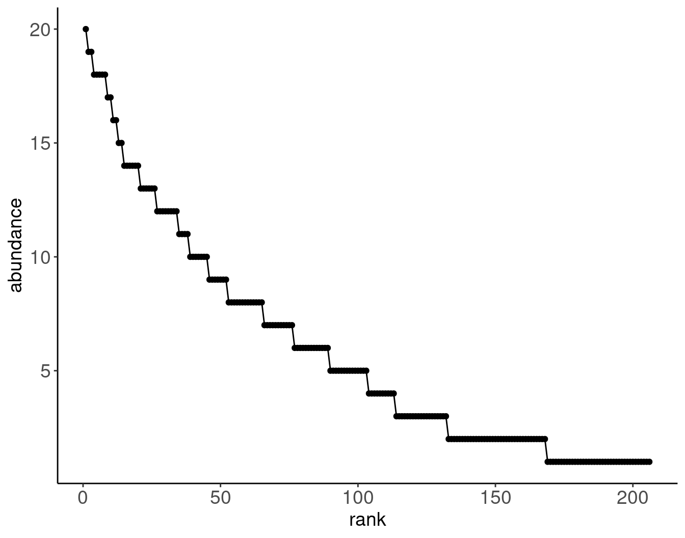
Example 2: Lepidoptera at a light trap in Maine, USA.

# Data transcribed from Bonson 1964, 'Patterns in the balance of nature and related problems in quantitative ecology'", accessed through archive.org

tribble(
  ~abundance, ~nsp,
  1,38,
  2,36,
  3,19,
  4,10,
  5,14,
  6,13,
  7,11,
  8,13,
  9,7,
  10,7,
  11,4,
  12,8,
  13,6,
  14,6,
  15,2,
  16,2,
  17,2,
  18,5,
  19,2,
  20,1
) |> 
  uncount(nsp) |> 
  mutate(spid = row_number()) |> 
  mutate(rank = rank(desc(abundance), ties.method = "first")) |> 
  ggplot(aes(x = rank, y = abundance)) +
  geom_point() + 
  geom_line() 

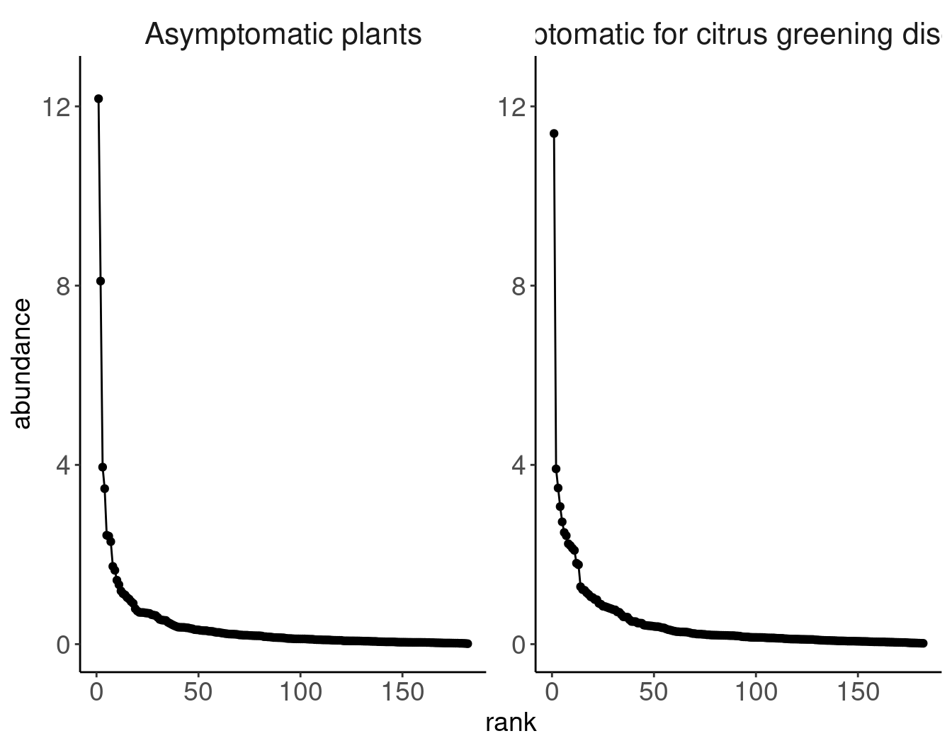
Example 3: Bacteria in citrus roots

# Data downloaded from supplement of 
# Blaustein et al. "Defining the Core Citrus Leaf- and Root-Associated Microbiota: Factors Associated with Community Structure and Implications for Managing Huanglongbing (Citrus Greening) Disease",
# https://doi.org/10.1128/AEM.00210-17

# First 46 rows have data from phyllosphere (leaf) bacteria
read_excel("hlb-microbes.xlsx", skip = 47) |> 
  dplyr::rename(meanabun_asym = 11, meanabun_sym = 13) |> 
  select(starts_with("meanabun_")) |> 
  pivot_longer(1:2, values_to = "abundance") |> 
  mutate(name = ifelse(name == "meanabun_asym", 
                       "Asymptomatic plants",
                       "Symptomatic for citrus greening disease")) |> 
  group_by(name) |> 
  mutate(rank = rank(desc(abundance), ties.method = "first")) |> 
  ggplot(aes(x = rank, y = abundance)) + 
  geom_point() + 
  geom_line() + 
  facet_wrap(.~name, scales = "free") + 
  ylim(0,12.5) + 
  theme(strip.text = element_text(size = 16))

Data from Blaustein et al. (link)

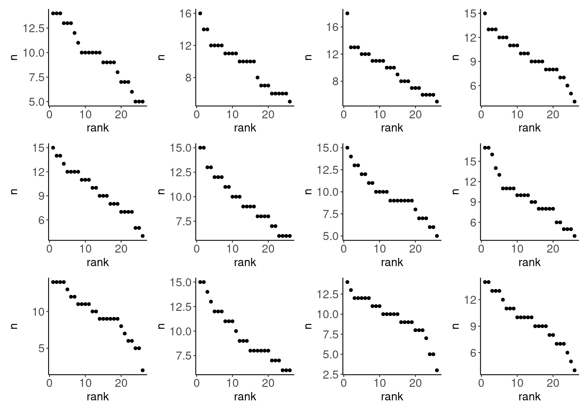
Example 4: Birds recorded at GKVK campus in 2024

# Uncomment the following lines to download data from ebird, 
# and add your ebird key
# library(rebird)
# gkvk_2024 <- tibble(date_format = na.omit(ymd(paste0("2024-",rep(1:12, each = 31),"-",01:31))),
#                     ebird_out = map(date_format,
#                                     ~ebirdhistorical(loc = 'L2525709', # for GKVK campus
#                                                      date = .x,
#                                                      key = "<your ebird key>")))

gkvk_2024 <- readRDS("gkvk_birds.rds")

list_rbind(gkvk_2024$ebird_out) |> 
  mutate(month = month(ymd_hm(obsDt), label = T, abbr = T)) |>
  group_by(comName,sciName,locName, month) |> 
  summarize(abundance = sum(howMany)) |> 
  ungroup() |>
  group_by(month) |> 
  mutate(rank = rank(desc(abundance), ties.method = "first")) |>
  ggplot(aes(x = rank, y = abundance)) + 
  geom_point(aes(group = comName)) + 
  geom_line(linewidth = 0.25) + 
  facet_wrap(.~month, scales = "free_x") + 
  xlim(0,140)
## `summarise()` has grouped output by 'comName', 'sciName', 'locName'. You can
## override using the `.groups` argument.
## Warning: Removed 42 rows containing missing values or values outside the scale range
## (`geom_point()`).

Think and discuss:

What might cause a species to be common or rare in a community?

What process(es) might give rise to this community-level pattern of a “long tail” in the distribution?

What could you do to test your hypothesis?

Pycnonotus jocosus (Red-whiskered Bulbul) photo by iNaturalist user karthik_83

Download PDF File

See also Wilson et al. “Biodiversity and species interactions: extending Lotka–Volterra community theory” (Link)

Today’s case study

Explaining patterns of species rarity and abundance in plant communities through plant–soil microbe interactions

Photo by a tallgrass prairie soil cross-section by Jim Richardson (link)

For additional details, see:
1. Bever et al. 1997, “Incorporating the Soil Community into Plant Population Dynamics: The Utility of the Feedback Approach” (link)
2. Kandlikar 2024, “Quantifying soil microbial effects on plant species coexistence: A conceptual synthesis” (link)

Mathematical expression of plant dynamics

\[\frac{dN_1}{dt} = w_1N_1 ~~~~ \text{and} ~~~ \frac{dN_2}{dt} = w_2N_2\]

\[w_i = m_{iA}f_A + m_{iB}(1-f_A)\]

where \(f_i\) is the relative frequency of microbial community \(i\) in the soil (e.g. \(f_A = \frac{N_A}{N_A+N_B}\))

Interpretation: Plants have exponential population growth at a rate determined by the composition of the soil community.

Mathematical expression of microbial dynamics

\[\frac{dN_A}{dt} = N_A\frac{N_1}{N_1 + N_2}~~~\text{and}~~~\frac{dN_B}{dt} = \nu N_B\frac{N_2}{N_1 + N_2}\]

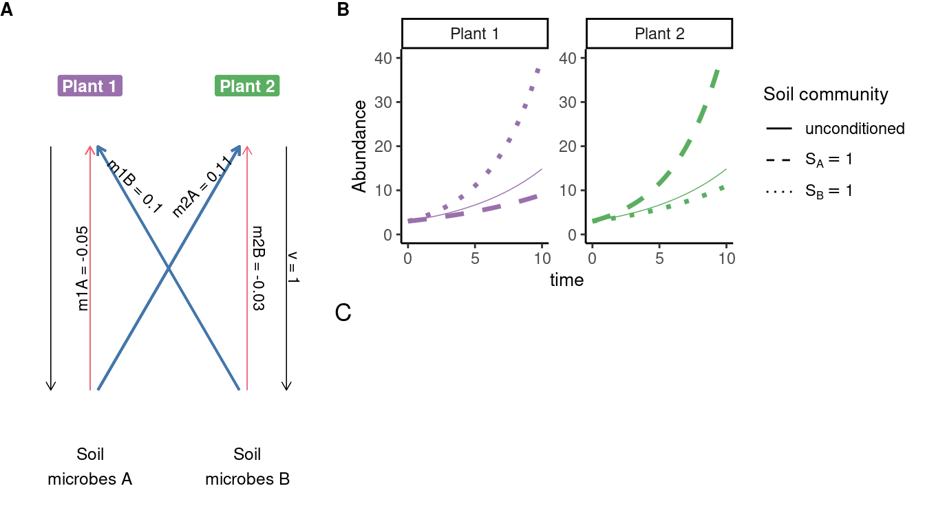
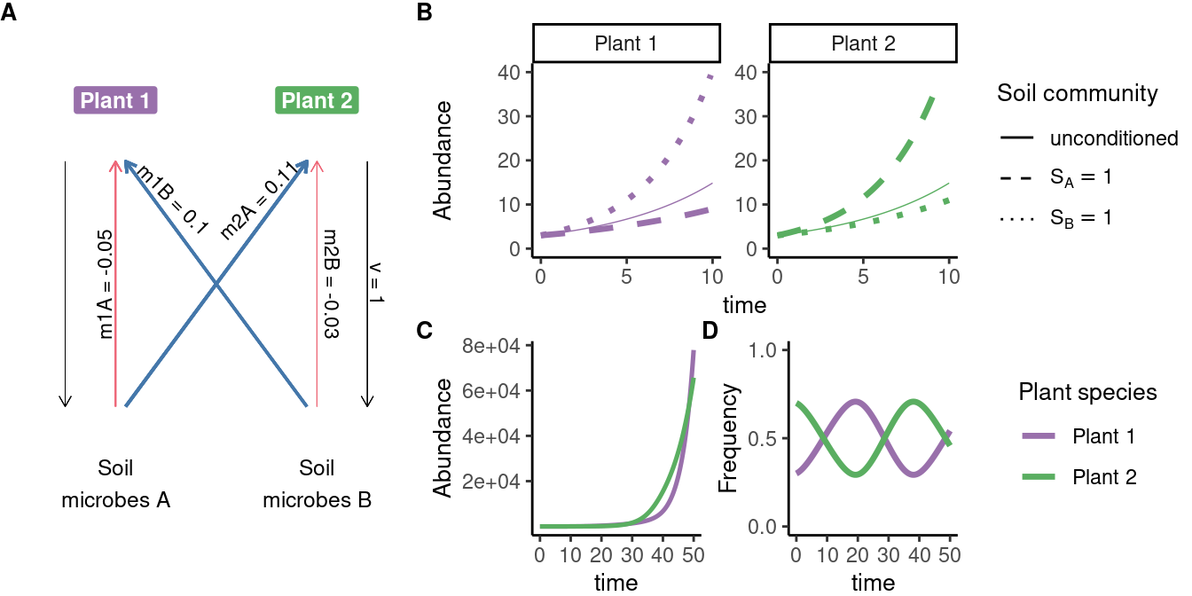
Interpretation: Soil communities grow at a rate determined by the frequency of each plant (and the relative strength of each plant’s conditioning effect, \(\nu\)).

Overview of model dynamics

• Plant population growth rates depend on the composition of the microbial community

• Microbial community composition in turn depends on the relative frequency of each plant.

• We can express the system’s dynamics in terms of plant and soil frequencies.

\[\frac{dF_1}{dt} = F_1(1-F_1)[(m_{1A}-m_{2A})F_A+(m_{1B}-m_{2B})(1-F_A)]\]

\[\frac{dF_A}{dt} = F_A(1-F_A)(F_A - \nu(1-F_A))\]

Download PDF File

Visualization of model dynamics

source("simulate-psf-model.R")
## Loading required package: deSolve
## Loading required package: rootSolve
## Loading required package: latex2exp
## 
## Attaching package: 'latex2exp'
## The following object is masked from 'package:plotly':
## 
##     TeX
## Warning: The `legend.text.align` argument of `theme()` is deprecated as of ggplot2
## 3.5.0.
## ℹ Please use theme(legend.text = element_text(hjust)) instead.
fig1_p1 <- fig1$p5
fig1_p1[[2]][[2]] = NULL
fig1_p1 
## Warning in geom_segment(aes(x = 0, xend = 0, y = 0.1, yend = 0.9), arrow = arrow(length = unit(0.03, : All aesthetics have length 1, but the data has 4 rows.
## ℹ Please consider using `annotate()` or provide this layer with data containing
##   a single row.
## Warning in geom_segment(aes(x = 0.05, xend = 0.95, y = 0.1, yend = 0.9), : All aesthetics have length 1, but the data has 4 rows.
## ℹ Please consider using `annotate()` or provide this layer with data containing
##   a single row.
## Warning in geom_segment(aes(x = 0.95, xend = 0.05, y = 0.1, yend = 0.9), : All aesthetics have length 1, but the data has 4 rows.
## ℹ Please consider using `annotate()` or provide this layer with data containing
##   a single row.
## Warning in geom_segment(aes(x = 1, xend = 1, y = 0.1, yend = 0.9), arrow = arrow(length = unit(0.03, : All aesthetics have length 1, but the data has 4 rows.
## ℹ Please consider using `annotate()` or provide this layer with data containing
##   a single row.
## Warning in geom_segment(aes(x = -0.25, xend = -0.25, y = 0.9, yend = 0.1), : All aesthetics have length 1, but the data has 4 rows.
## ℹ Please consider using `annotate()` or provide this layer with data containing
##   a single row.
## Warning in geom_segment(aes(x = 1.25, xend = 1.25, y = 0.9, yend = 0.1), : All aesthetics have length 1, but the data has 4 rows.
## ℹ Please consider using `annotate()` or provide this layer with data containing
##   a single row.
## Warning in is.na(x): is.na() applied to non-(list or vector) of type
## 'expression'
## Warning in is.na(x): is.na() applied to non-(list or vector) of type
## 'expression'
## Warning in is.na(x): is.na() applied to non-(list or vector) of type
## 'expression'
## Warning in is.na(x): is.na() applied to non-(list or vector) of type
## 'expression'
## Warning: Removed 6 rows containing missing values or values outside the scale range
## (`geom_line()`).

Visualization of model dynamics

fig1$p5
## Warning in geom_segment(aes(x = 0, xend = 0, y = 0.1, yend = 0.9), arrow = arrow(length = unit(0.03, : All aesthetics have length 1, but the data has 4 rows.
## ℹ Please consider using `annotate()` or provide this layer with data containing
##   a single row.
## Warning in geom_segment(aes(x = 0.05, xend = 0.95, y = 0.1, yend = 0.9), : All aesthetics have length 1, but the data has 4 rows.
## ℹ Please consider using `annotate()` or provide this layer with data containing
##   a single row.
## Warning in geom_segment(aes(x = 0.95, xend = 0.05, y = 0.1, yend = 0.9), : All aesthetics have length 1, but the data has 4 rows.
## ℹ Please consider using `annotate()` or provide this layer with data containing
##   a single row.
## Warning in geom_segment(aes(x = 1, xend = 1, y = 0.1, yend = 0.9), arrow = arrow(length = unit(0.03, : All aesthetics have length 1, but the data has 4 rows.
## ℹ Please consider using `annotate()` or provide this layer with data containing
##   a single row.
## Warning in geom_segment(aes(x = -0.25, xend = -0.25, y = 0.9, yend = 0.1), : All aesthetics have length 1, but the data has 4 rows.
## ℹ Please consider using `annotate()` or provide this layer with data containing
##   a single row.
## Warning in geom_segment(aes(x = 1.25, xend = 1.25, y = 0.9, yend = 0.1), : All aesthetics have length 1, but the data has 4 rows.
## ℹ Please consider using `annotate()` or provide this layer with data containing
##   a single row.
## Warning in is.na(x): is.na() applied to non-(list or vector) of type
## 'expression'
## Warning in is.na(x): is.na() applied to non-(list or vector) of type
## 'expression'
## Warning in is.na(x): is.na() applied to non-(list or vector) of type
## 'expression'
## Warning in is.na(x): is.na() applied to non-(list or vector) of type
## 'expression'
## Warning: Removed 6 rows containing missing values or values outside the scale range
## (`geom_line()`).

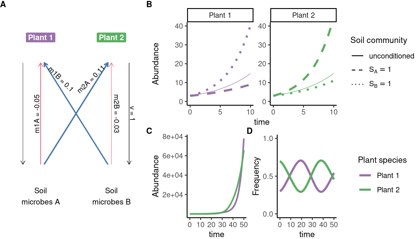
Under this set of parameters, the frequencies of the species oscillate - a form of neutral coexistence.

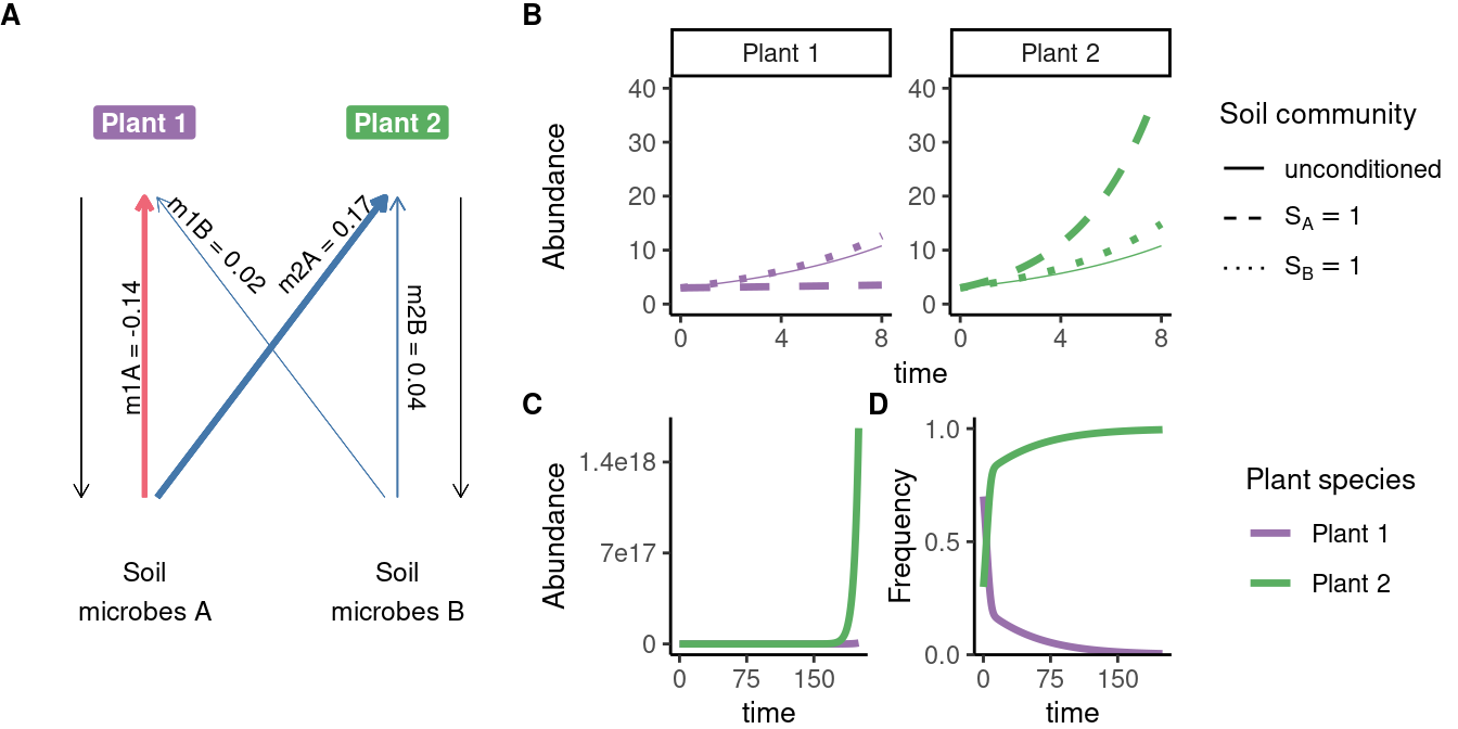
Visualization of model dynamics

fig2AtoD
## Warning in geom_segment(aes(x = 0, xend = 0, y = 0.1, yend = 0.9), arrow = arrow(length = unit(0.03, : All aesthetics have length 1, but the data has 4 rows.
## ℹ Please consider using `annotate()` or provide this layer with data containing
##   a single row.
## Warning in geom_segment(aes(x = 0.05, xend = 0.95, y = 0.1, yend = 0.9), : All aesthetics have length 1, but the data has 4 rows.
## ℹ Please consider using `annotate()` or provide this layer with data containing
##   a single row.
## Warning in geom_segment(aes(x = 0.95, xend = 0.05, y = 0.1, yend = 0.9), : All aesthetics have length 1, but the data has 4 rows.
## ℹ Please consider using `annotate()` or provide this layer with data containing
##   a single row.
## Warning in geom_segment(aes(x = 1, xend = 1, y = 0.1, yend = 0.9), arrow = arrow(length = unit(0.03, : All aesthetics have length 1, but the data has 4 rows.
## ℹ Please consider using `annotate()` or provide this layer with data containing
##   a single row.
## Warning in geom_segment(aes(x = -0.25, xend = -0.25, y = 0.9, yend = 0.1), : All aesthetics have length 1, but the data has 4 rows.
## ℹ Please consider using `annotate()` or provide this layer with data containing
##   a single row.
## Warning in geom_segment(aes(x = 1.25, xend = 1.25, y = 0.9, yend = 0.1), : All aesthetics have length 1, but the data has 4 rows.
## ℹ Please consider using `annotate()` or provide this layer with data containing
##   a single row.
## Warning in is.na(x): is.na() applied to non-(list or vector) of type
## 'expression'
## Warning in is.na(x): is.na() applied to non-(list or vector) of type
## 'expression'
## Warning in is.na(x): is.na() applied to non-(list or vector) of type
## 'expression'
## Warning in is.na(x): is.na() applied to non-(list or vector) of type
## 'expression'
## Warning: Removed 122 rows containing missing values or values outside the scale range
## (`geom_line()`).

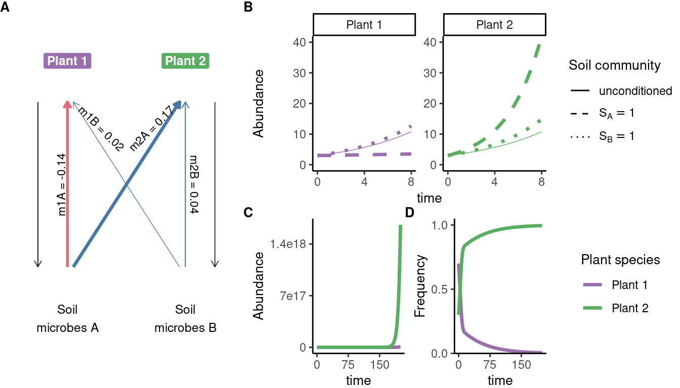
Under other parameters, the frequency of one species reaches 1 - a form of species exclusion.

What determines the outcome of these interactions?

Original analysis emphasized the role of species–specific pathogens (or mutualists that favor the non-host species)

What determines the outcome of these interactions?

Original analysis emphasized the role of species–specific pathogens (or mutualists that favor the non-host species)

Mathematically,

\[ \overbrace{(m_{1A} + m_{2B})}^{\text{intraspecific effects}} - \overbrace{(m_{1B} + m_{2A})}^{\text{interspecific effects}} < 0\]

What determines the outcome of these interactions?

Original analysis emphasized the role of species–specific pathogens (or mutualists that favor the non-host species)

Mathematically,

\[ \underbrace{\overbrace{(m_{1A} + m_{2B})}^{\text{intraspecific effects}} - \overbrace{(m_{1B} + m_{2A})}^{\text{interspecific effects}}}_{I_S} < 0 \]

Let’s reflect:

In what ways is this model similar to or different from the Lotka-Volterra framework?

What biological processes are included in the model, and what are missing?

Lasting influence of the Bever model

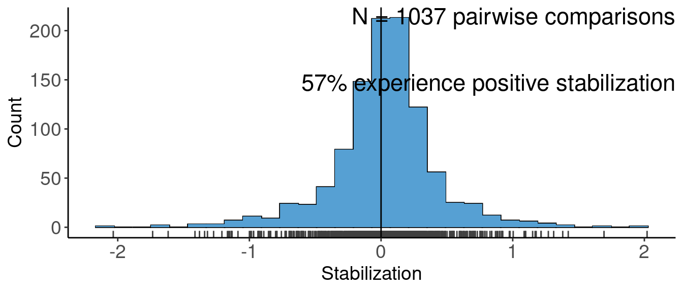
# Dataset downloaded from Figshare: 
# curl::curl_download("https://figshare.com/ndownloader/files/14874749", destfile = "crawford-supplement.xlsx")

read_excel("crawford-supplement.xlsx", sheet = "Data") |> 
  mutate(stab = -0.5*rrIs) |> # show in terms of stabilization instead of I_s
  filter(stab > -3) |> 
  ggplot(aes(x = stab)) + 
  geom_histogram(color = "black") +
  geom_histogram(fill = "#56A0D3") +
  geom_rug(color = "grey25") + 
  geom_vline(xintercept = 0) + 
  annotate("text", x = Inf, y = Inf, label = "N = 1037 pairwise comparisons\n
           57% experience positive stabilization",
           vjust=1, hjust = 1, size = 6) +
  xlab("Stabilization") + ylab("Count")
## `stat_bin()` using `bins = 30`. Pick better value with `binwidth`.
## `stat_bin()` using `bins = 30`. Pick better value with `binwidth`.

Data from Crawford et al. 2019 (link)

How does this relate to species commonness and rarity?

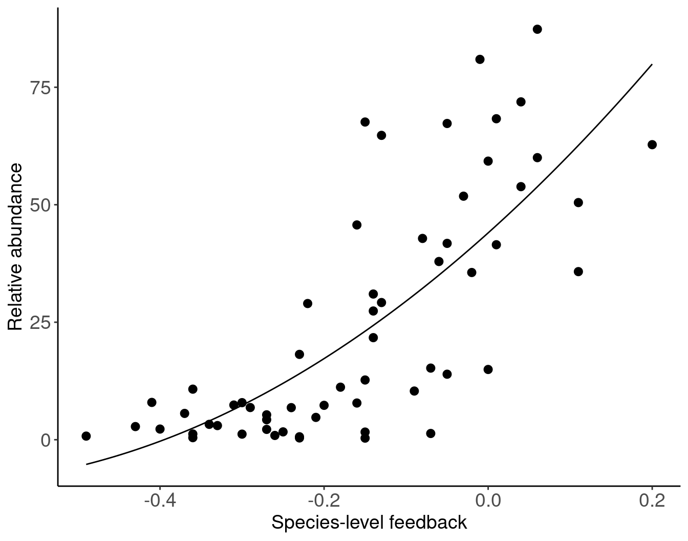
“In 1997, a big change happened in my approach to studying plant–microbe interactions. While attending the Mycological Society of America meeting in Montreal, I listened to Jim Bever talk about a simple but powerful framework on plant–soil feedback. He showed how his concept could be used to study plant and microbial effects and responses at the same time.”

John Klironomos, in The Paper Trail

# data extracted from Fig. 3 of Klironomos 2002, https://www.nature.com/articles/417067a.pdf
# using WebPlotDigitizer
tribble(
  ~fb, ~abun,
  -0.34, 3.27,
  -0.41, 7.94,
  -0.27, 2.20,
  0.01, 41.49,
  -0.14, 27.39,
  -0.05, 67.29,
  0.00, 59.28,
  -0.16, 7.81,
  0.11, 35.77,
  -0.08, 42.83,
  -0.15, 1.63,
  -0.36, 1.22,
  -0.07, 1.33,
  -0.27, 5.30,
  -0.40, 2.27,
  0.06, 87.34,
  -0.21, 4.75,
  -0.23, 0.38,
  -0.02, 35.58,
  -0.05, 41.78,
  -0.25, 1.67,
  -0.20, 7.32,
  -0.15, 12.71,
  -0.09, 10.36,
  -0.18, 11.18,
  0.04, 53.85,
  -0.29, 6.85,
  -0.14, 31.00,
  -0.33, 3.01,
  -0.07, 15.24,
  -0.15, 67.60,
  0.00, 14.95,
  -0.22, 28.98,
  0.11, 50.46,
  -0.03, 51.82,
  -0.23, 18.16,
  -0.15, 0.34,
  -0.36, 0.44,
  -0.30, 1.19,
  0.20, 62.78,
  -0.30, 7.89,
  -0.14, 21.72,
  -0.37, 5.60,
  -0.13, 64.76,
  -0.26, 0.91,
  -0.16, 45.70,
  -0.24, 6.83,
  -0.43, 2.80,
  -0.13, 29.19,
  -0.49, 0.77,
  -0.05, 13.94,
  -0.06, 37.92,
  0.01, 68.30,
  -0.36, 10.76,
  -0.31, 7.38,
  -0.27, 4.26,
  0.06, 60.02,
  0.04, 71.89,
  -0.23, 0.63,
  -0.01, 80.93,
) |> 
  ggplot(aes(x = fb, y = abun)) + 
  geom_point(size = 2.5) + 
  # fit line from Fig 3 of the paper
  geom_function(fun = function(x) 114.529*x^2 + 156.652*x + 44.013) + 
  xlab("Species-level feedback") + 
  ylab("Relative abundance") 

Species–level feedback calculated as (approx.)

feedback_i = biomass_i in soil i - biomass_i in other soil

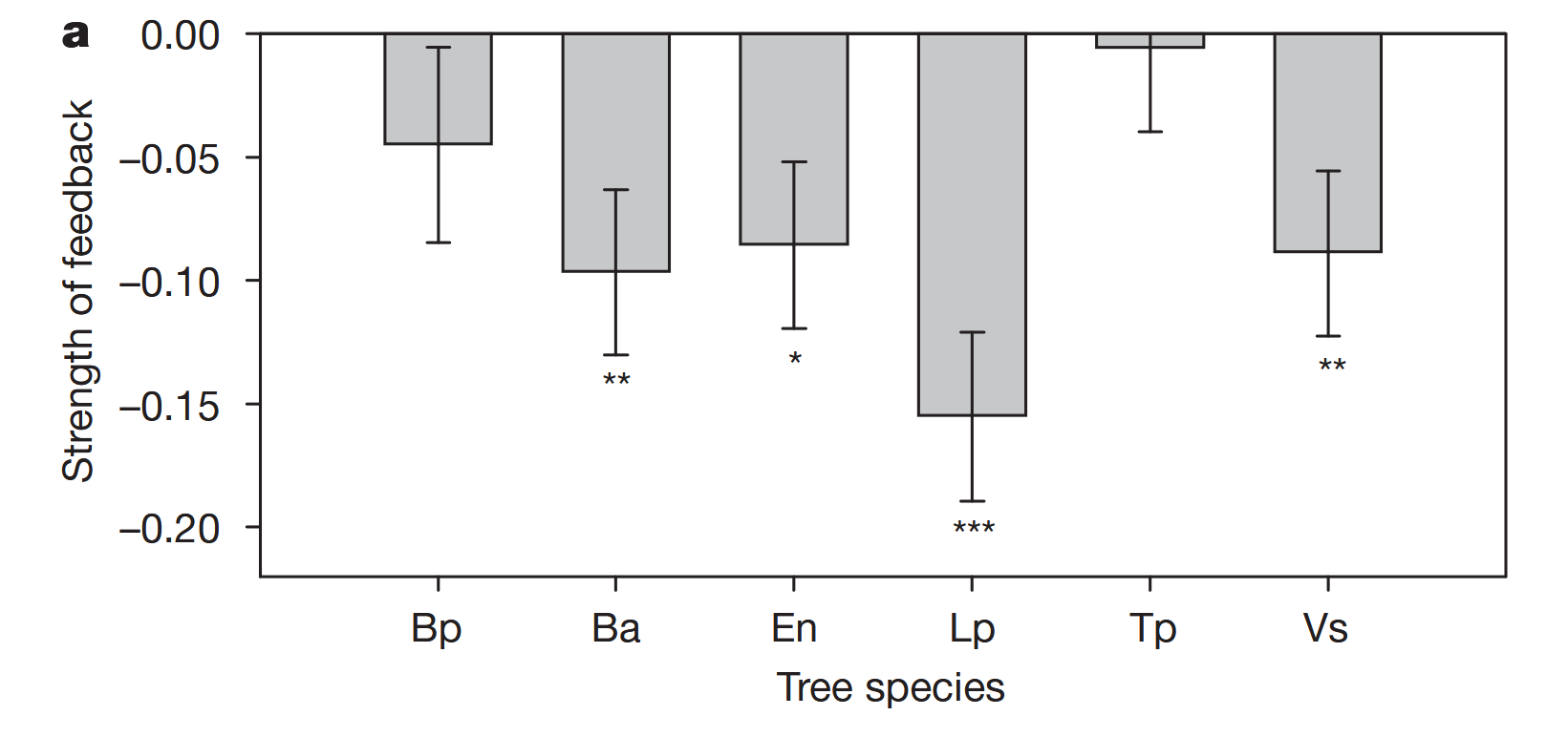
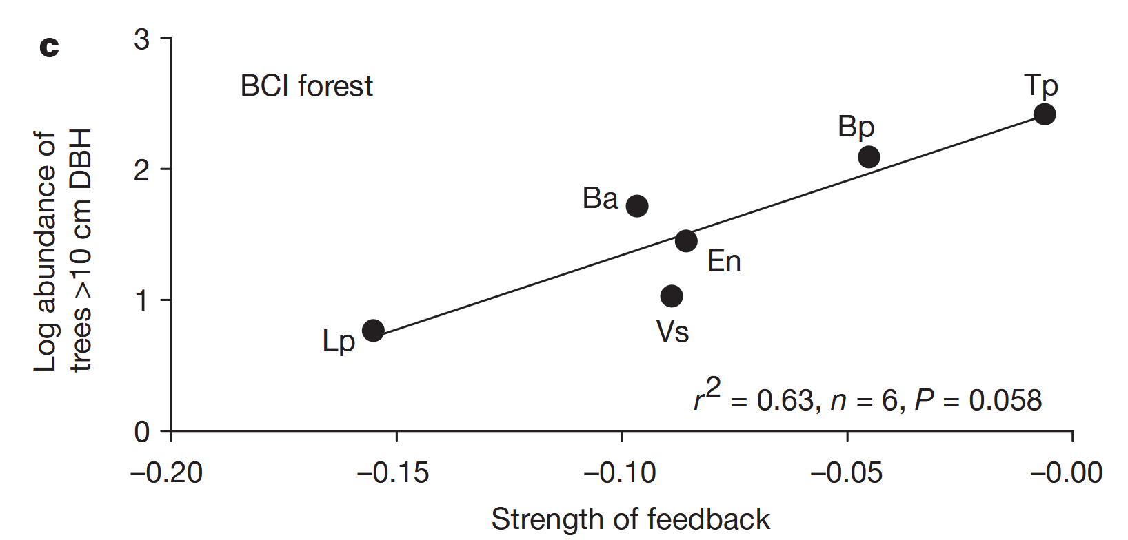
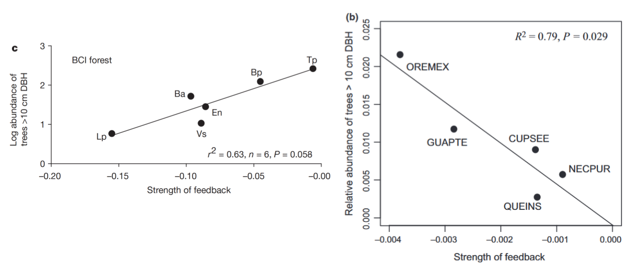
Approach: Shade-house studies of pairwise feedback among 6 species of varying abundances, and a complementary field transplant experiment. (Shade-house study with soils from BCI; field study in another nearby forest).

Experimentally quantified pairwise feedback (\(I_S\)) between \({6 \choose 2} = 15\) pairs of species.

mangan_species <- c("Brosimum.alicastrum","Beilschmiedia.pendula", "Eugenia.nesiotica", "Lacmellea.panamensis", "Tetragastris.panamensis", "Virola.surinamensis")
p_mangan <- 
  bci_ranks |> 
  mutate(in_mangan = ifelse(species %in% mangan_species, "yes", "no")) |> 
  ggplot(aes(x = rank, y = abundance)) +
  geom_line(linewidth = 0.1) +
  geom_point(aes(group = species, color = in_mangan, size = in_mangan)) +
  scale_color_manual(values = c("grey", "black")) +
  scale_size_manual(values = c(0.75,2)) + 
  theme(legend.position = "none")

ggplotly(p_mangan) |> config(displayModeBar = FALSE)

For each focal species, calculate the average of all \(I_S\) involving that species:

Key result: Species involved in more stabilized interactions (more negative \(I_S\)) tend to be less abundant in the forest

Complementary field study provided further support

“Our [studies] reinforce the conclusion that trees are abundant because they are less susceptible to the detrimental effects of their associated soil communities than are rarer tree species. Thus, localized negative plant–soil feedback occurring between plants and below-ground organisms may be a general mechanism for the maintenance of plant species diversity and patterns of relative abundance across ecosystems ranging from temperate grasslands to tropical forests.”

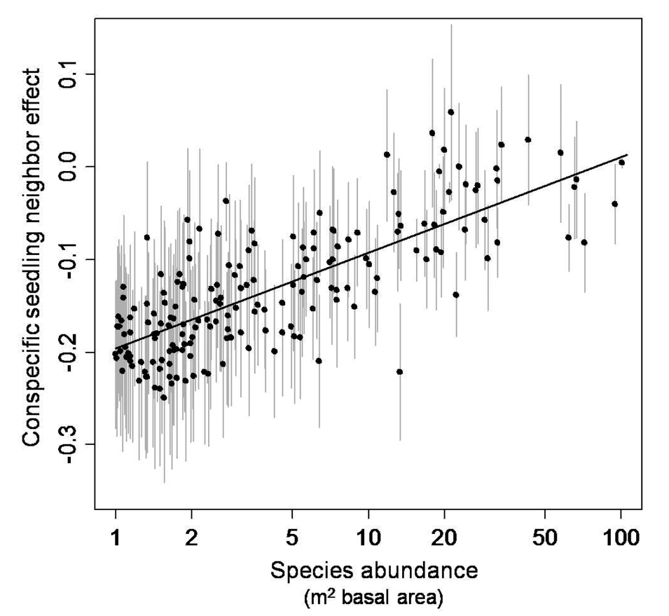
Approach: Statistical analysis of seedling census data from BCI to evlauate the factors that determine seedling survival.

Key result: Species that have stronger self-limitation in seedling recruitment are less common as adults in the forest.

Understanding the drivers of species abundance is critical for identifying and protecting rare species that have an inherently higher risk of extinction. Previous effort to identify key traits that correlate with species rarity have had limited success. The results here suggest that such studies should look beyond morphological and physiological traits to include species sensitivity to biotic interactions, namely, the degree to which species inhibit their own regeneration.

Let’s reflect:

What is the conceptual argument built up through these studies?

Do you think this is a strong mechanistic explanation?

What more evidence would you like to see to further support or reject this hypothesis?

A wrinkle in the story

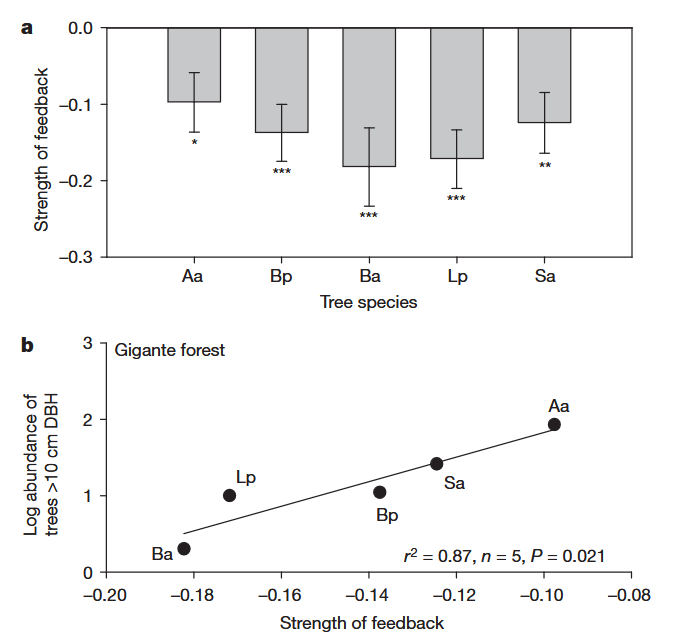
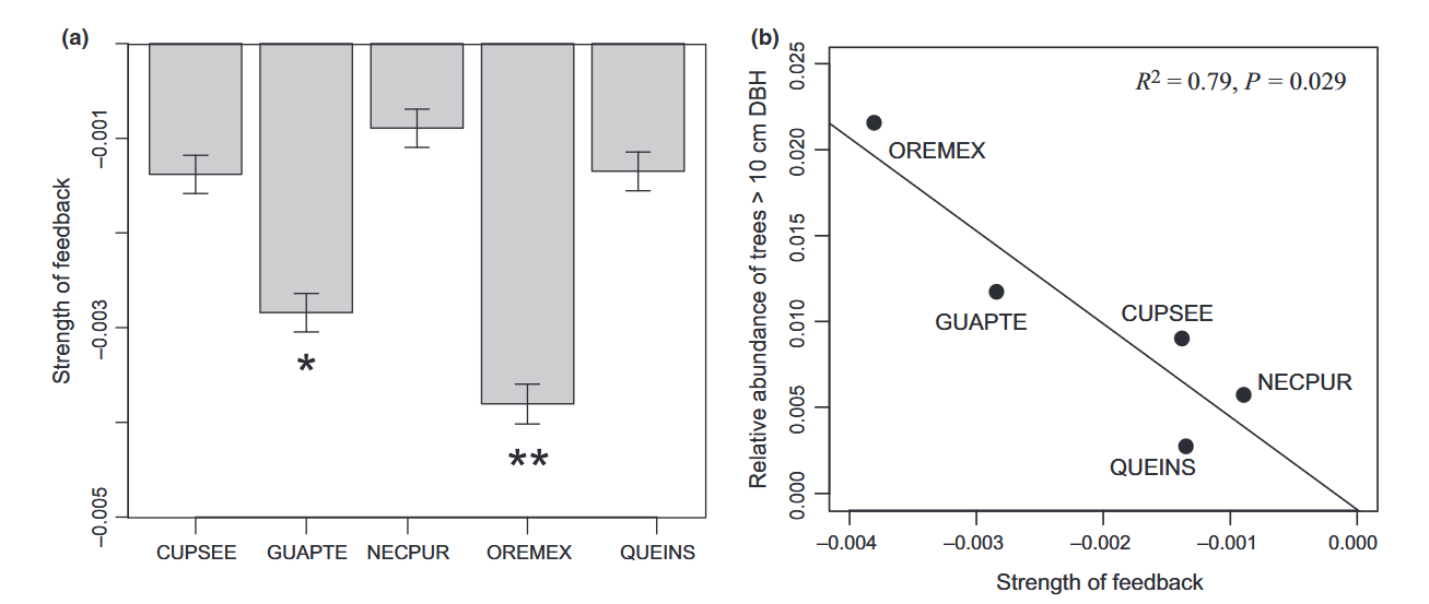
Approach: Shade-house study of pairwise feedback among 5 species of varying abundances, along with extensive field evaluation of mycorrhizal associations. Work done in lower montane tropical forests in Panama.

Key result: Species involved in more stabilized interactions (more negative \(I_S\)) tend to be more abundant in forests

Contrasting relationships across two nearby forests

“This result contrasts with findings from lowland tropical forest and temperate grasslands, where more abundant species show weaker negative PSF. This is the first PSF experiment ever done including montane tree species and more research in this topic is needed to confirm if this is widespread phenomenon of just a peculiarity of our system.”

Summary of timeline

• 1997: Bever’s feedback model, which suggested an experiment design and metric of stabilization
  
• 2002: Klironomos’ study, correlating microbial responses to abundance in a temperate old field
• 2010: Mangan et al.’s study, correlating strength of pairwise feedback to abundance in a tropical forest
• 2010: Comita et al.’s study, correlating strength of neighborhood effect to abundance in the same tropical forest
• 2016: Corrales et al.’s study, finding the opposite correlation between strength of pairwise feedback and abundance in a tropical montane forest

Let’s reflect:

What do you think might be happening here?

Theoretical advances in feedback theory

Recall that the original analysis in 1997 emphasized the strength of intra- vs. interspecific interactions:

\[ \underbrace{\overbrace{(m_{1A} + m_{2B})}^{\text{intraspecific effects}} - \overbrace{(m_{1B} + m_{2A})}^{\text{interspecific effects}}}_{I_S} < 0 \]

\(I_S\) does not fully capture microbial effects, even in this simple model

For details, see Ke and Miki (2015); Kandlikar et al. (2019); Broekman et al. (2019); Beckman et al. (2023); Kandlikar (2024)

With equivalent values of \(I_S\), vastly different model dynamics are possible.

fig1$p5
## Warning in geom_segment(aes(x = 0, xend = 0, y = 0.1, yend = 0.9), arrow = arrow(length = unit(0.03, : All aesthetics have length 1, but the data has 4 rows.
## ℹ Please consider using `annotate()` or provide this layer with data containing
##   a single row.
## Warning in geom_segment(aes(x = 0.05, xend = 0.95, y = 0.1, yend = 0.9), : All aesthetics have length 1, but the data has 4 rows.
## ℹ Please consider using `annotate()` or provide this layer with data containing
##   a single row.
## Warning in geom_segment(aes(x = 0.95, xend = 0.05, y = 0.1, yend = 0.9), : All aesthetics have length 1, but the data has 4 rows.
## ℹ Please consider using `annotate()` or provide this layer with data containing
##   a single row.
## Warning in geom_segment(aes(x = 1, xend = 1, y = 0.1, yend = 0.9), arrow = arrow(length = unit(0.03, : All aesthetics have length 1, but the data has 4 rows.
## ℹ Please consider using `annotate()` or provide this layer with data containing
##   a single row.
## Warning in geom_segment(aes(x = -0.25, xend = -0.25, y = 0.9, yend = 0.1), : All aesthetics have length 1, but the data has 4 rows.
## ℹ Please consider using `annotate()` or provide this layer with data containing
##   a single row.
## Warning in geom_segment(aes(x = 1.25, xend = 1.25, y = 0.9, yend = 0.1), : All aesthetics have length 1, but the data has 4 rows.
## ℹ Please consider using `annotate()` or provide this layer with data containing
##   a single row.
## Warning in is.na(x): is.na() applied to non-(list or vector) of type
## 'expression'
## Warning in is.na(x): is.na() applied to non-(list or vector) of type
## 'expression'
## Warning in is.na(x): is.na() applied to non-(list or vector) of type
## 'expression'
## Warning in is.na(x): is.na() applied to non-(list or vector) of type
## 'expression'
## Warning: Removed 6 rows containing missing values or values outside the scale range
## (`geom_line()`).

With equivalent values of \(I_S\), vastly different model dynamics are possible.

fig2AtoD
## Warning in geom_segment(aes(x = 0, xend = 0, y = 0.1, yend = 0.9), arrow = arrow(length = unit(0.03, : All aesthetics have length 1, but the data has 4 rows.
## ℹ Please consider using `annotate()` or provide this layer with data containing
##   a single row.
## Warning in geom_segment(aes(x = 0.05, xend = 0.95, y = 0.1, yend = 0.9), : All aesthetics have length 1, but the data has 4 rows.
## ℹ Please consider using `annotate()` or provide this layer with data containing
##   a single row.
## Warning in geom_segment(aes(x = 0.95, xend = 0.05, y = 0.1, yend = 0.9), : All aesthetics have length 1, but the data has 4 rows.
## ℹ Please consider using `annotate()` or provide this layer with data containing
##   a single row.
## Warning in geom_segment(aes(x = 1, xend = 1, y = 0.1, yend = 0.9), arrow = arrow(length = unit(0.03, : All aesthetics have length 1, but the data has 4 rows.
## ℹ Please consider using `annotate()` or provide this layer with data containing
##   a single row.
## Warning in geom_segment(aes(x = -0.25, xend = -0.25, y = 0.9, yend = 0.1), : All aesthetics have length 1, but the data has 4 rows.
## ℹ Please consider using `annotate()` or provide this layer with data containing
##   a single row.
## Warning in geom_segment(aes(x = 1.25, xend = 1.25, y = 0.9, yend = 0.1), : All aesthetics have length 1, but the data has 4 rows.
## ℹ Please consider using `annotate()` or provide this layer with data containing
##   a single row.
## Warning in is.na(x): is.na() applied to non-(list or vector) of type
## 'expression'
## Warning in is.na(x): is.na() applied to non-(list or vector) of type
## 'expression'
## Warning in is.na(x): is.na() applied to non-(list or vector) of type
## 'expression'
## Warning in is.na(x): is.na() applied to non-(list or vector) of type
## 'expression'
## Warning: Removed 122 rows containing missing values or values outside the scale range
## (`geom_line()`).

Think back to how \(I_S\) was derived - what does it guarantee?

• \(I_S<0\) suggests neutral stability (in frequency space)

• But doesn’t indicate a feasible equilibrium.

Download PDF File

A feasible equilibrium with neutral stability requires:

\[m_{2B}<m_{1B} ~~~ \text{and} ~~~ m_{1A}<m_{2A}\]

We can also arrive at this requirement through invasion analysis

• Growth rate of species \(i\) into an equilibrium monoculture of species \(j\)
  • \(\frac{dF_i}{dt}|_{F_j = 1}\) (“Invasion growth rate”)
  • Species coexistence if \(\frac{dF_1}{dt}|_{F_2 = 1} > 0\) and \(\frac{dF_2}{dt}|_{F_1 = 1} > 0\)

Independent exercise: Derive the criteria for coexistence in the Bever 1997 model through analyzing feasibility analysis and through invasion analysis.

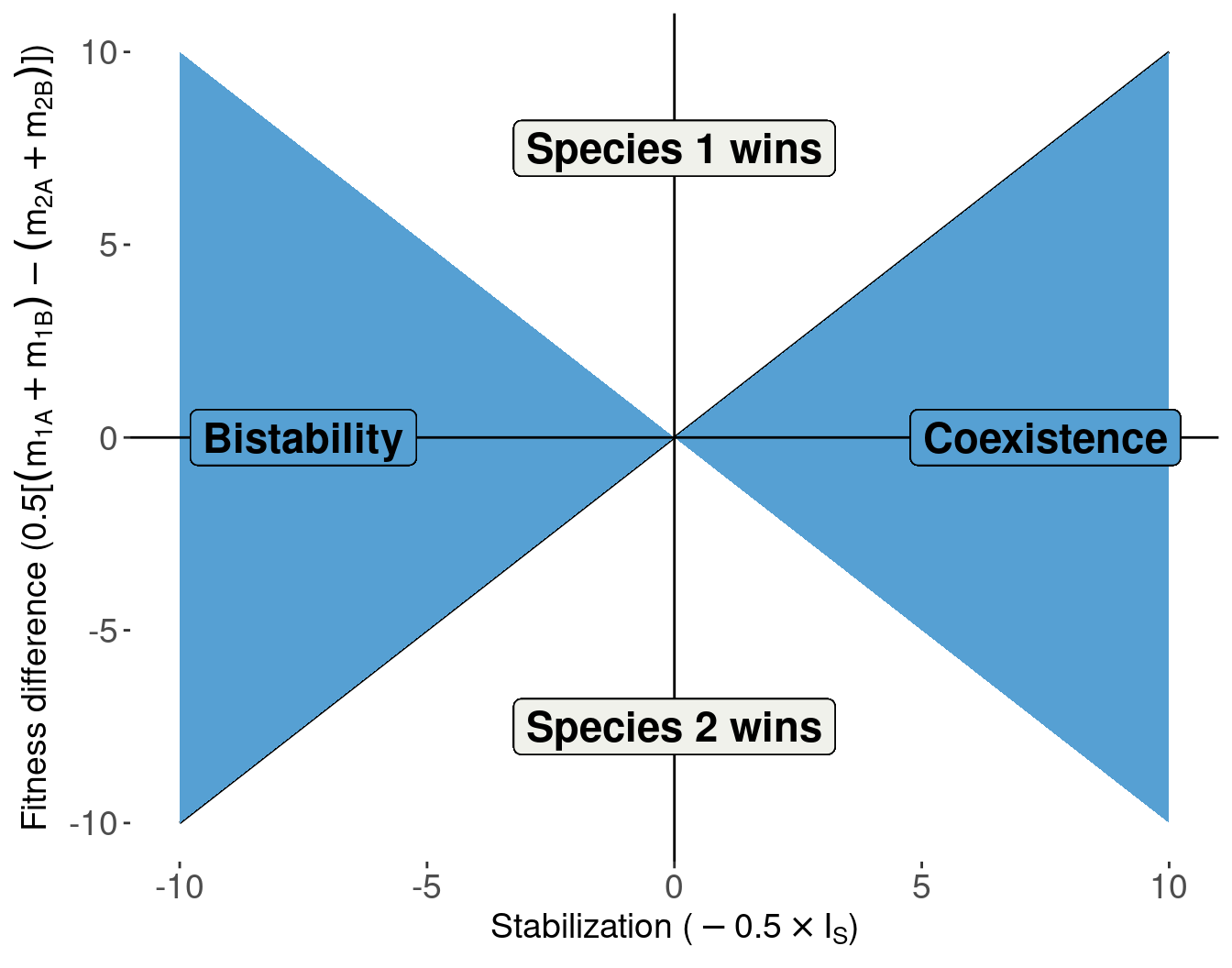
We can also express this in the “Chesson” language

• Decompose the invasion growth rates into the strength of stabilization and fitness differences.

tibble(x = seq(-10,10),
       y = seq(-10,10)) |> 
  ggplot(aes(x = x, y = y)) + 
  geom_line() + 
  geom_ribbon(aes(ymin = -y, ymax = y), fill = "#56A0D3") +
  geom_hline(yintercept = 0) +
  geom_vline(xintercept = 0) + 
  geom_label(x = 7.5, y = 0, label = "Coexistence", fontface = "bold", size = 6,  inherit.aes = F, fill = "#56A0D3") + 
    geom_label(x = -7.5, y = 0, label = "Bistability", fontface = "bold", size = 6,  inherit.aes = F, fill = "#56A0D3") + 
  geom_label(x = 0, y = 7.5, label = "Species 1 wins", fontface = "bold", size = 6, fill = "#F0F1EB",  inherit.aes = F) + 
  geom_label(x = 0, y = -7.5, label = "Species 2 wins", fontface = "bold", size = 6, fill = "#F0F1EB",  inherit.aes = F) + 

  xlab(latex2exp::TeX("Stabilization ($-0.5 \\times I_S$)")) + 
  ylab(latex2exp::TeX("Fitness difference ($0.5  [(m_{1A} + m_{1B}) - (m_{2A} + m_{2B})]$)")) + 
  theme(axis.line = element_blank())

Empirically, microbially-mediated fitness differences tend to outweight stabilizing effects

(Data shown for 72 out of >500 species pairs in the meta-analysis)

Open question:

Is variation in relative abundance better explained by variation in species’ overall responses to microbes (fitness imbalance) than to “self vs. other” microbes (stabilization)?

The Bever 1997 framework does not permit multispecies coexistence

Here, we extend this canonical model of PSFs to include an arbitrary number of plant species and analyse the dynamics. Surprisingly, we find that coexistence of more than two species is virtually impossible, suggesting that alternative theoretical frameworks are needed to describe feedbacks observed in diverse natural communities.

The [abundance] projected onto [frequency] dynamics can mask unbiological outcomes in the original model (e.g. relative abundances oscillate around equilibrium while absolute abundances shrink to zero or explode to infinity).

Indeed, the absolute abundance model used to derive our species frequency dynamics does not generally possess any fixed point, which is a basic requirement for species coexistence.

Our analysis suggests that the internal dynamics of plant or soil communities must interact with PSFs to maintain diversity in natural systems.

Multispecies coexistence becomes possible when plants, soils, or both experience an independent source of self-regulation, which might arise from resource competition, physical limits to density or some other mechanism.

Download PDF File

Resources and readings

General readings on the dialogue between theoretical and empirical approaches to studying nature

• Levins, 1966, “The Strategy of Model Building in Population Biology”, https://www.jstor.org/stable/27836590
  
• Levins and Lewontin, 1980, “Dialectics and reductionism in ecology”, https://doi.org/10.1007/BF00413856
• Pielou, 1981, “The Usefulness of Ecological Models: A Stock-Taking”, https://www.jstor.org/stable/pdf/2826368.pdf
• Odenbaugh, 2005. “Idealized, inaccurate but successful: A pragmatic approach to evaluating models in theoretical ecology”. https://doi.org/10.1007/s10539-004-0478-6
• Marquet et al, “On Theory in Ecology”. 2015, https://doi.org/10.1093/biosci/biu098
• Grainger et al. 2022. “An Empiricist’s Guide to Using Ecological Theory”, https://doi.org/10.1086/717206
• Shaw, et al. 2024, “Six personas to adopt when framing theoretical research questions in biology”, https://doi.org/10.1098/rspb.2024.0803

Plant–soil microbe interactions

• Bever et al. 1997, “Incorporating the Soil Community into Plant Population Dynamics: The Utility of the Feedback Approach” https://www.jstor.org/stable/2960528
• Bever 2003, “Soil community feedback and the coexistence of competitors: conceptual frameworks and empirical tests”, https://doi.org/10.1046/j.1469-8137.2003.00714.x
• Ke and Wan 2019, “Effects of soil microbes on plant competition: a perspective from modern coexistence theory” https://doi.org/10.1002/ecm.1391
• Miller et al. 2022, “No robust multispecies coexistence in a canonical model of plant–soil feedbacks”, https://doi.org/10.1111/ele.14027
• Kandlikar 2024, “Quantifying soil microbial effects on plant species coexistence: A conceptual synthesis” https://doi.org/10.1002/ajb2.16316

Other explanations for variation in species abundances

• McGill et al. 2007, “Species abundance distributions: moving beyond single prediction theories to integration within an ecological framework”, https://doi.org/10.1111/j.1461-0248.2007.01094.x
• Wilson et al. 2004 “Biodiversity and species interactions: extending Lotka–Volterra community theory”, https://doi.org/10.1046/j.1461-0248.2003.00521.x
• Hubbell 2001, “Unified Theory of Biodiversity and Biogeography”, https://archive.org/details/unifiedneutralth0000hubb
• McGill, 2003, “A test of the unified neutral theory of biodiversity”, https://doi.org/10.1038/nature01583

Contact

Gaurav Kandlikar: gkandlikar@lsu.edu
Meghna Krishnadas: meghnak@ncbs.res.in