Approach


Lasting influence of the Bever model
Code
# Dataset downloaded from Figshare:
# curl::curl_download("https://figshare.com/ndownloader/files/14874749", destfile = "../crawford-supplement.xlsx")

read_excel("../data/crawford-supplement.xlsx", sheet = "Data") |>
  mutate(stab = -0.5*rrIs) |> # show in terms of stabilization instead of I_s
  filter(stab > -3) |> # Remove the pair with Stab approx. 6 -- according to McCarthy Neuman (original author), this is likely due to bad seed survival
  ggplot(aes(x = stab)) +
  geom_histogram(color = "black") +
  geom_histogram(fill = "#56A0D3") +
  geom_rug(color = "grey25") +
  geom_vline(xintercept = 0) +
  annotate("text", x = Inf, y = Inf, label = "N = 1037 pairwise comparisons\n
           57% experience positive stabilization",
           vjust=1, hjust = 1, size = 6) +
  xlab("Stabilization") + ylab("Count")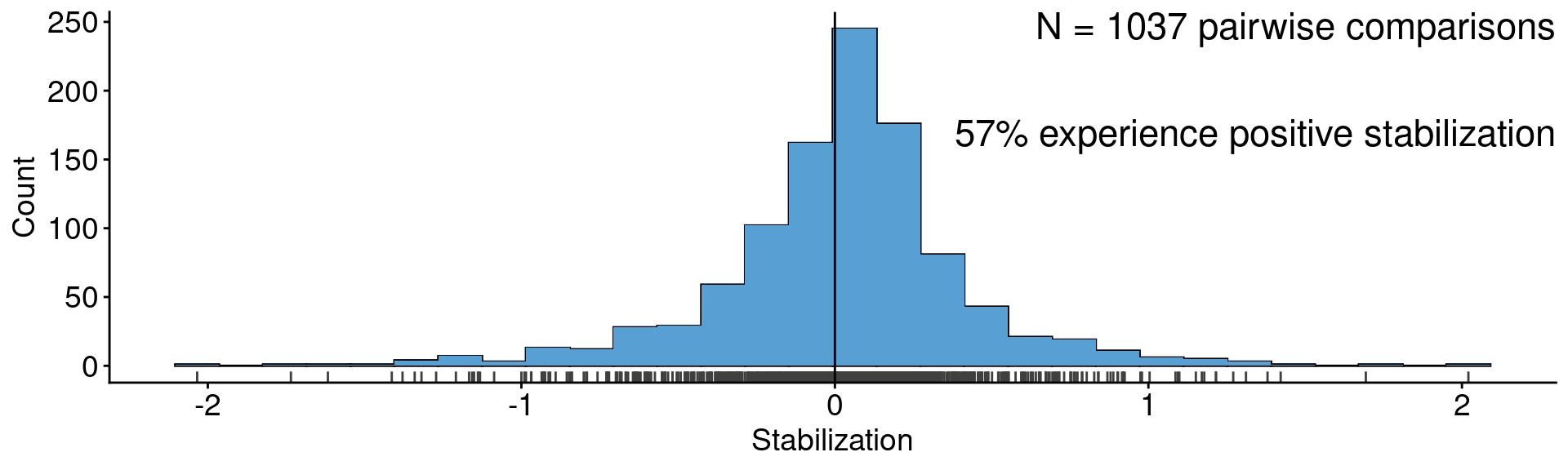
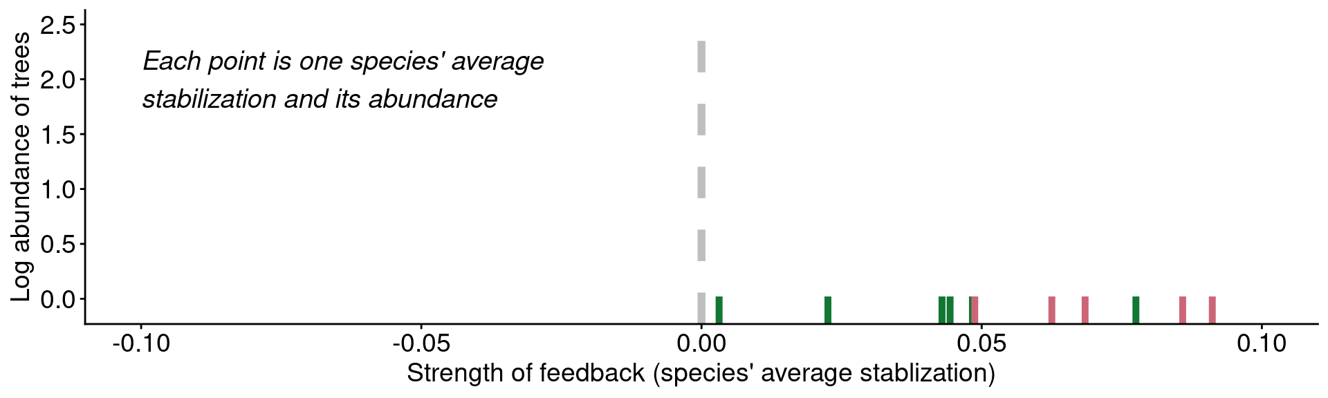
Data from Crawford et al. (2019)
Microbial feedbacks drive community patterns?
Code
mangan <-
tribble(~IS, ~abun, ~where,
-0.15504664970313828, 0.7732558139534884, "BCI",
-0.0887192536047498, 1.005813953488372, "BCI",
-0.08583545377438509, 1.4825581395348837, "BCI",
-0.09669211195928756, 1.7267441860465116, "BCI",
-0.04512298558100089, 2.1104651162790695, "BCI",
-0.006276505513146763, 2.4186046511627906, "BCI",
-0.18231106613816006, 0.3003106037506997, "Gigante",
-0.1717428991693779, 1.0202629577384568, "Gigante",
-0.13691306110550813, 1.083509520825865, "Gigante",
-0.1250429718781308, 1.425445047930817, "Gigante",
-0.09753373250550346, 1.9673983333947622, "Gigante") |>
mutate(stab = IS*-0.5)
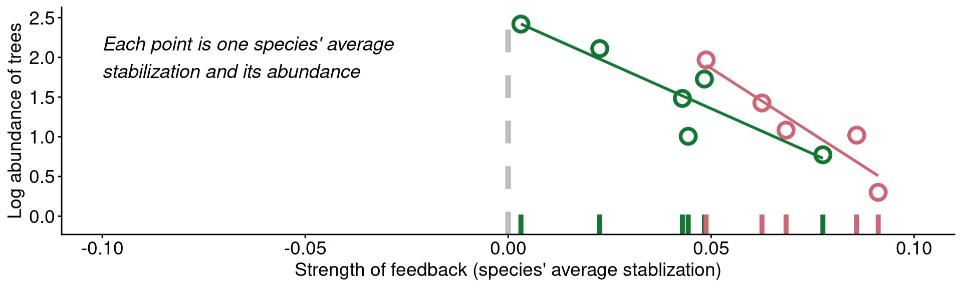
mangan_rug_blank <-
mangan |>
ggplot(aes(x = stab,y = abun, color = where)) +
# geom_rug(sides = 'b', linewidth = 2) +
# geom_point(size = 4, stroke = 2, shape = 21) +
# geom_smooth(method = "lm", se = F) +
geom_point(color = 'transparent') +
scale_color_manual(values = c("#117733", "#cc6677")) +
geom_vline(xintercept = 0, linetype = 'dashed', color = 'grey', linewidth = 2) +
xlab("Strength of feedback (species' average stablization)") +
ylab("Log abundance of trees") +
theme(legend.position = 'none') +
scale_x_continuous(limits = c(-0.1, 0.1))+
scale_y_continuous(limits = c(-0.1,2.5))
mangan_rug_blank
Data from Mangan et al. (2010)
Microbial feedbacks drive community patterns?
Code

Data from Mangan et al. (2010)
Microbial feedbacks drive community patterns?
Code
Data from Mangan et al. (2010)
Microbial feedbacks drive community patterns?
Code
Data from Mangan et al. (2010)
Microbial feedbacks drive community patterns?
Code
mangan_rug +
    geom_point(size = 4, stroke = 2, shape = 21) +
  geom_smooth(method = "lm", se = F) +
  annotate('text', x = -0.1, y = 2, fontface = "italic", hjust = 0, vjust = 0.5, size = 5,
             label = '"[...] trees are abundant because they are less\nsusceptible to the detrimental effects of\ntheir associated soil communities than are\nrarer tree species"')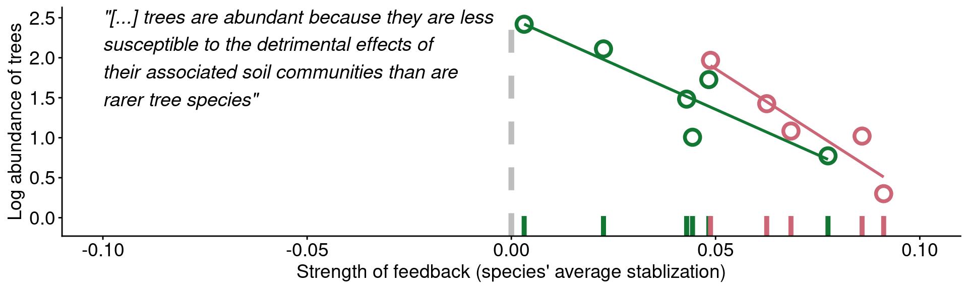
Data from Mangan et al. (2010)
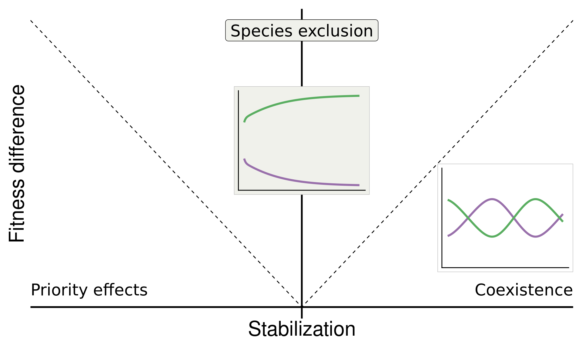
A puzzle: same stabilization, different model dynamics
Code
# Define a function used for making the PSF framework
# schematic, given a set of parameter values
make_params_plot <- function(params, scale = 1.5) {

  color_func <- function(x) {
    ifelse(x < 0, "#EE6677", "#4477AA")
  }
  df <- data.frame(x = c(0,0,1,1),
                   y = c(0,1,0,1),
                   type = c("M", "P", "M", "P"))

  params_plot <-
    ggplot(df) +
    annotate("text", x = 0, y = 1.1, size = 3.25, label = "Plant 1",
             color = "black", fill = "#9970ab", fontface = "bold") +
    annotate("text", x = 1, y = 1.1, size = 3.25, label = "Plant 2",
             color = "black", fill = "#5aae61", fontface = "bold") +
    annotate("text", x = 0, y = -0.15, size = 3.25,
             label = "Soil\nmicrobes A", label.size = 0, fill = "transparent") +
    annotate("text", x = 1, y = -0.15, size = 3.25,
             label = "Soil\nmicrobes B", label.size = 0, fill = "transparent") +
    annotate("text", x = 0.45, y = -0.4, size = 3.5, fill = "transparent",
               label.size = 0.05,
               label = (paste0("Stabilization = ",
                                  0.5*(params["m1B"] + params["m2A"] - params["m1A"] - params["m2B"])))) +
    geom_segment(aes(x = 0, xend = 0, y = 0.1, yend = 0.9),
                 arrow = arrow(length = unit(0.03, "npc")),
                 linewidth = abs(params["m1A"])*scale,
                 color = alpha(color_func(params["m1A"]), 1)) +
    geom_segment(aes(x = 0.05, xend = 0.95, y = 0.1, yend = 0.9),
                 arrow = arrow(length = unit(0.03, "npc")),
                 linewidth = abs(params["m2A"])*scale,
                 color = alpha(color_func(params["m1B"]),1)) +
    geom_segment(aes(x = 0.95, xend = 0.05, y = 0.1, yend = 0.9),
                 arrow = arrow(length = unit(0.03, "npc")),
                 linewidth = abs(params["m1B"])*scale,
                 color = alpha(color_func(params["m2A"]), 1)) +
    geom_segment(aes(x = 1, xend = 1, y = 0.1, yend = 0.9),
                 arrow = arrow(length = unit(0.03, "npc"),),
                 linewidth = abs(params["m2B"])*scale,
                 color = alpha(color_func(params["m2B"]), 1)) +

    # Plant cultivation of microbes
    geom_segment(aes(x = -0.25, xend = -0.25, y = 0.9, yend = 0.1),
                 linewidth = 0.15, linetype = 1,
                 arrow = arrow(length = unit(0.03, "npc"))) +
    geom_segment(aes(x = 1.25, xend = 1.25, y = 0.9, yend = 0.1),
                 linewidth = 0.15, linetype = 1,
                 arrow = arrow(length = unit(0.03, "npc"))) +

    annotate("text", x = 0, y = 0.5,
             label = (paste0("m1A = ", params["m1A"])),
             angle = 90, vjust = -0.25, size = 3) +
    annotate("text", x = 1.15, y = 0.5,
             label = (paste0("m2B = ", params["m2B"])),
             angle = -90, vjust = 1.5, size = 3) +
    annotate("text", x = 0.75, y = 0.75,
             label = (paste0("m2A = ", params["m2A"])),
             angle = 45, vjust = -0.25, size = 3) +
    annotate("text", x = 0.25, y = 0.75,
             label = (paste0("m1B = ", params["m1B"])),
             angle = -45, vjust = -0.25, size = 3) +
    xlim(c(-0.4, 1.4)) +
    coord_cartesian(ylim = c(-0.25, 1.15), clip = "off") +
    theme_void() +
    theme(legend.position = "none",
          plot.caption = element_text(hjust = 0.5, size = 10))
  return(params_plot)
}

# Define a function for simulating the dynamics of the
# PSF model with deSolve
params_coex <- c(m10 = 0.16, m20 = 0.16,
                 m1A = 0.11, m1B = 0.26,
                 m2A = 0.27, m2B = 0.13, v = 1)

time <- seq(0,50,0.1)
init_pA_05 <- c(N1 = 3, N2 = 7, p1 = 0.3, pA = 0.3)
out_pA_05 <- ode(y = init_pA_05, times = time, func = psf_model, parms = params_coex) |> data.frame()


params_to_plot_coex <- c(m1A = unname(params_coex["m1A"]-params_coex["m10"]),
                         m1B = unname(params_coex["m1B"]-params_coex["m10"]),
                         m2A = unname(params_coex["m2A"]-params_coex["m20"]),
                         m2B = unname(params_coex["m2B"]-params_coex["m20"]), v=1)
param_plot_coex <-
  make_params_plot(params_to_plot_coex, scale = 6) +
  annotate("text", x = 1.375, y = 0.5,
           label = paste0("v = ", params_coex["v"]),
           angle = -90, vjust = 1.5, size = 3)

panel_abund_coex <-
  out_pA_05 |>
  as_tibble() |>
  select(time, N1, N2) |>
  pivot_longer(N1:N2) |>
  ggplot(aes(x = time, y = value, color = name)) +
  geom_line(linewidth = 0.9) +
  scale_color_manual(values = c("#9970ab", "#5aae61"),
                     name = "Plant species", label = c("Plant 1", "Plant 2"), guide = "none") +
  scale_y_continuous(breaks = c(2e4, 4e4, 6e4, 8e4), labels = scales::scientific) +
  ylab("Abundance") +
  theme(axis.title = element_text(size = 10))

# Panel D: plot for frequencies of both plants when growing
# in dynamic soils
panel_freq_coex <-
  out_pA_05 |>
  as_tibble() |>
  mutate(p2 = 1-p1) |>
  select(time, p1, p2) |>
  pivot_longer(p1:p2) |>
  ggplot(aes(x = time, y = value, color = name)) +
  geom_line(linewidth = 1.2) +
  scale_color_manual(values = c("#9970ab", "#5aae61"),
                     name = "Plant species", label = c("Plant 1", "Plant 2")) +
  scale_y_continuous(limits = c(0,1), breaks = c(0, 0.5, 1)) +
  ylab("Frequency") +
  theme(axis.title = element_text(size = 10))

param_plot_coex +  {panel_abund_coex+panel_freq_coex &
  theme(axis.text = element_text(size = 8), legend.position = 'none')} +
  plot_layout(widths = c(1/3, 2/3))
Code
# Define a function for simulating the dynamics of the
# PSF model with deSolve
params <- c(m10 = 0.16, m20 = 0.16,
              m1A = 0.02, m2A = 0.33,
              m1B = 0.18, m2B = 0.20, v = 1)

time <- seq(0,200,0.1)
init_pA_05 <- c(N1 = 3, N2 = 7, p1 = 0.3, pA = 0.3)
out_pA_05 <- ode(y = init_pA_05, times = time, func = psf_model, parms = params) |> data.frame()


params_to_plot <- c(m1A = unname(params["m1A"]-params["m10"]),
                    m1B = unname(params["m1B"]-params["m10"]),
                    m2A = unname(params["m2A"]-params["m20"]),
                    m2B = unname(params["m2B"]-params["m20"]), v=1)
param_plot <-
  make_params_plot(params_to_plot, scale = 6) +
  annotate("text", x = 1.375, y = 0.5,
           label = paste0("v = ", params["v"]),
           angle = -90, vjust = 1.5, size = 3)

panel_abund <-
  out_pA_05 |>
  as_tibble() |>
  select(time, N1, N2) |>
  pivot_longer(N1:N2) |>
  ggplot(aes(x = time, y = value, color = name)) +
  geom_line(linewidth = 0.9) +
  scale_color_manual(values = c("#9970ab", "#5aae61"),
                     name = "Plant species", label = c("Plant 1", "Plant 2"), guide = "none") +
    scale_y_continuous(breaks = c(0,8e17,1.6e18), labels = c("0", "7e17","1.4e18")) +
  ylab("Abundance")

# Panel D: plot for frequencies of both plants when growing
# in dynamic soils
panel_freq <-
  out_pA_05 |>
  as_tibble() |>
  mutate(p2 = 1-p1) |>
  select(time, p1, p2) |>
  pivot_longer(p1:p2) |>
  ggplot(aes(x = time, y = value, color = name)) +
  geom_line(linewidth = 1.2) +
  scale_color_manual(values = c("#9970ab", "#5aae61"),
                     name = "Plant species", label = c("Plant 1", "Plant 2")) +
  scale_y_continuous(limits = c(0,1), breaks = c(0, 0.5, 1)) +
  ylab("Frequency")

param_plot + {panel_abund + panel_freq &
  theme(axis.text = element_text(size = 8), legend.position = 'none')} +
  plot_layout(widths = c(1/3, 2/3))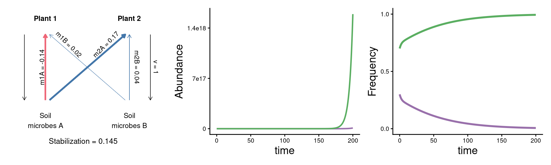
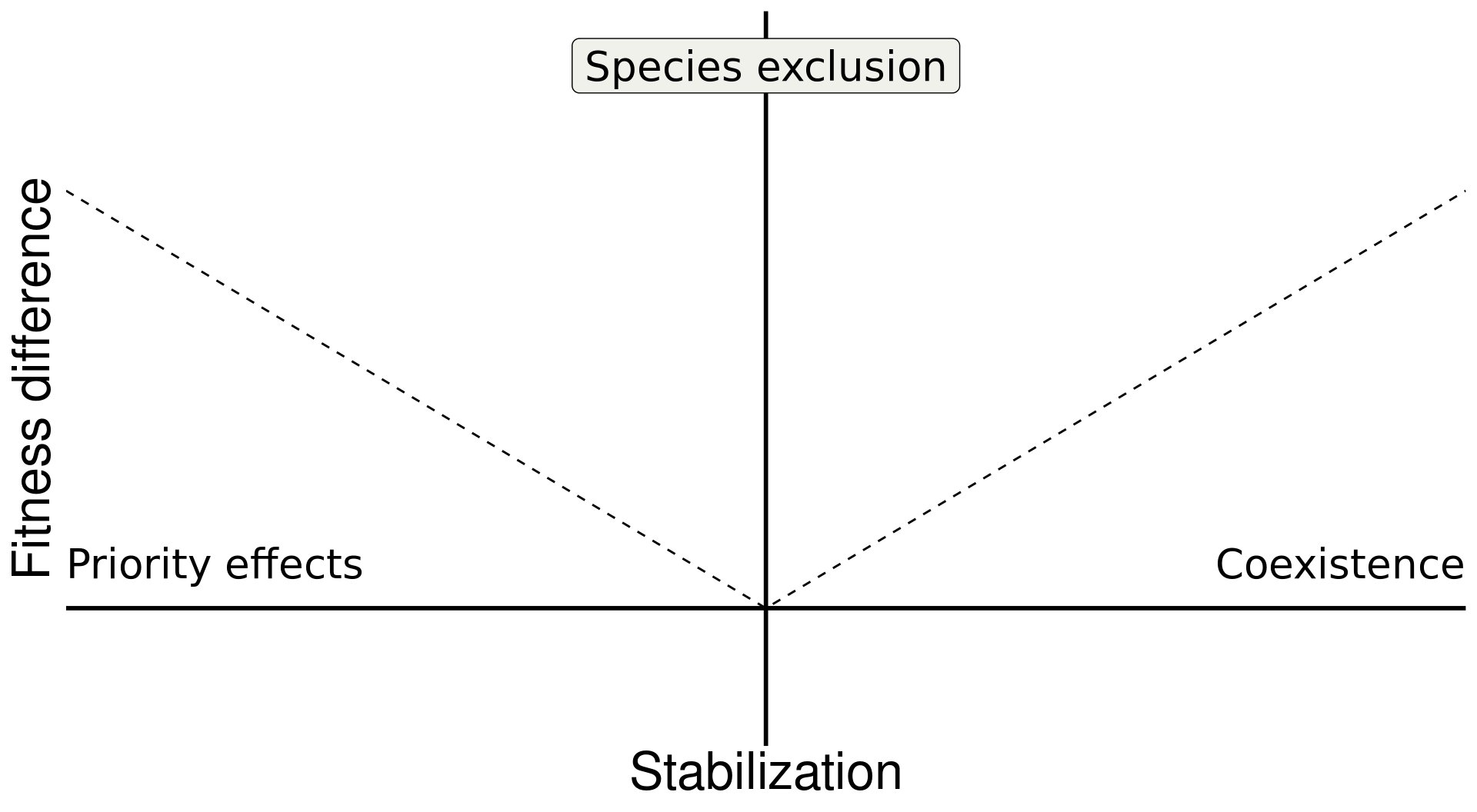
How can we more accurately infer predicted plant coexistence under plant–soil feedback?
Build on insights from coexistence theory (Chesson 2018):
Stabilization is necessary for coexistence but doesn’t guarantee coexistence
Stable coexistence is possible only when stabilization overcomes competitive imbalances (fitness differences)

How can we more accurately infer predicted plant dynamics under plant–soil feedback?

How can we more accurately infer predicted plant dynamics under plant–soil feedback?
How can we more accurately infer predicted plant dynamics under plant–soil feedback?

How can we more accurately infer predicted plant dynamics under plant–soil feedback?


Code
base <-
  tibble(sd = seq(-1,1,0.1),
       fd = c(seq(1,0,-0.1), seq(0.1,1,0.1))) |>
  ggplot(aes(x = sd, y = fd)) +
  geom_line(linetype = "dashed") +
  geom_hline(yintercept = 0, linewidth = 1) +
  geom_vline(xintercept = 0, linewidth = 1) +
  xlab("Stabilization") +
  ylab("Fitness difference") +
  theme(axis.text = element_blank(),
        axis.ticks = element_blank(),
        axis.line = element_blank(),
        axis.title = element_text(size = 25)) +
  scale_x_continuous(expand = c(0,0)) +
  scale_y_continuous(expand = c(0.04,0))
base
Code
base <-
base +
  annotate("text", x = Inf, y = 0, hjust = 1, vjust = -1,
           label = "Coexistence", size = 7, family = "italic") +
  annotate("text", x = -Inf, y = 0, hjust = 0, vjust = -1,
           label = "Priority effects", size = 7, family = "italic") +
  annotate("label", x = 0, y = Inf,  vjust = 1.5,
           label = "Species exclusion", size = 7, fill = "#F0F1EB", family = "italic")

base
Code
metrics <- function(params) {
  IS <- with(as.list(params), {m1A - m2A - m1B + m2B})
  FD <- with(as.list(params), {(1/2)*(m1A+m2A) - (1/2)*(m1B+m2B)})
  SD <- (-1/2)*IS
  return(c(IS = IS, SD = SD, FD = FD))
}

coex_metrics <- metrics(params_coex)
base_coex <-
  base +
  inset_element({panel_freq_coex + theme(legend.position = 'none',
                                         axis.text = element_blank(),
                                         axis.ticks = element_blank(),
                                         axis.title = element_blank(),
                                         plot.background = element_rect(color = "grey"))},
                0.75,0.15,1,0.5)
base_coex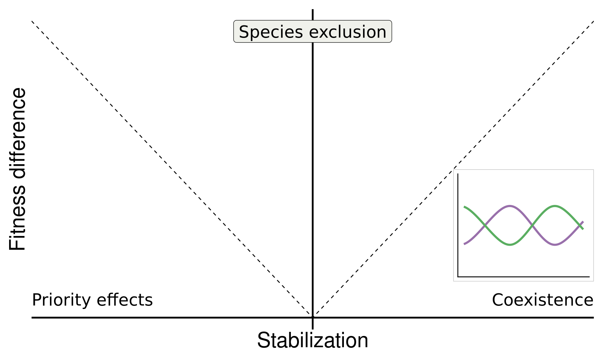


Code
# Dataset downloaded from Figshare:
# curl::curl_download("https://datadryad.org/downloads/file_stream/367188", destfile = "../data/kandlikar2021-supplement.csv")

biomass_wide <-
  read_csv("../data/kandlikar2021-supplement.csv") |>
  mutate(log_agb = log(abg_dry_g)) |>
  mutate(source_soil = ifelse(source_soil == "aastr", "str", source_soil),
                source_soil = ifelse(source_soil == "abfld", "fld", source_soil),
                pair = paste0(source_soil, "_", focal_species)) |>
      select(replicate, pair, log_agb)  |>
    pivot_wider(names_from = pair, values_from = log_agb) |>
  filter(!is.na(replicate))

# Calculate the Stabilization between each species pair ----
# Recall that following the definition of the m terms in Bever 1997,
# and the analysis of this model in Kandlikar 2019,
# stablization = -0.5*(log(m1A) + log(m2B) - log(m1B) - log(m2A))
# Here is a function that does this calculation
# (recall that after the data reshaping above,
# each column represents a given value of log(m1A))
calculate_stabilization <- function(df) {
  df |>
    # In df, each row is one repilcate/rack, and each column
    # represents the growth of one species in one soil type.
    # e.g. "FE_ACWR" is the growth of FE in ACWR-cultivated soil.
    mutate(AC_FE = -0.5*(AC_ACWR - AC_FEMI - FE_ACWR + FE_FEMI),
           AC_HO = -0.5*(AC_ACWR - AC_HOMU - HO_ACWR + HO_HOMU),
           AC_SA = -0.5*(AC_ACWR - AC_SACO - SA_ACWR + SA_SACO),
           AC_PL = -0.5*(AC_ACWR - AC_PLER - PL_ACWR + PL_PLER),
           AC_UR = -0.5*(AC_ACWR - AC_URLI - UR_ACWR + UR_URLI),
           FE_HO = -0.5*(FE_FEMI - FE_HOMU - HO_FEMI + HO_HOMU),
           FE_SA = -0.5*(FE_FEMI - FE_SACO - SA_FEMI + SA_SACO),
           FE_PL = -0.5*(FE_FEMI - FE_PLER - PL_FEMI + PL_PLER),
           FE_UR = -0.5*(FE_FEMI - FE_URLI - UR_FEMI + UR_URLI),
           HO_PL = -0.5*(HO_HOMU - HO_PLER - PL_HOMU + PL_PLER),
           HO_SA = -0.5*(HO_HOMU - HO_SACO - SA_HOMU + SA_SACO),
           HO_UR = -0.5*(HO_HOMU - HO_URLI - UR_HOMU + UR_URLI),
           SA_PL = -0.5*(SA_SACO - SA_PLER - PL_SACO + PL_PLER),
           SA_UR = -0.5*(SA_SACO - SA_URLI - UR_SACO + UR_URLI),
           PL_UR = -0.5*(PL_PLER - PL_URLI - UR_PLER + UR_URLI)) |>
    select(replicate, AC_FE:PL_UR) |>
    gather(pair, stabilization, AC_FE:PL_UR)
}

stabilization_values <- calculate_stabilization(biomass_wide)
# Seven values are NA; we can omit these
stabilization_values <- stabilization_values |>
  filter(!(is.na(stabilization)))

# Calculating the Fitness difference between each species pair ----
# Similarly, we can now calculate the fitness difference between
# each pair. Recall that FD = 0.5*(log(m1A)+log(m1B)-log(m2A)-log(m2B))
# But recall that here, IT IS IMPORTANT THAT
# m1A = (m1_soilA - m1_fieldSoil)!

# The following function does this calculation:
calculate_fitdiffs <- function(df) {
  df |>
    mutate(AC_FE = 0.5*((AC_ACWR-fld_ACWR) + (FE_ACWR-fld_ACWR) - (AC_FEMI-fld_FEMI) - (FE_FEMI-fld_FEMI)),
           AC_HO = 0.5*((AC_ACWR-fld_ACWR) + (HO_ACWR-fld_ACWR) - (AC_HOMU-fld_HOMU) - (HO_HOMU-fld_HOMU)),
           AC_SA = 0.5*((AC_ACWR-fld_ACWR) + (SA_ACWR-fld_ACWR) - (AC_SACO-fld_SACO) - (SA_SACO-fld_SACO)),
           AC_PL = 0.5*((AC_ACWR-fld_ACWR) + (PL_ACWR-fld_ACWR) - (AC_PLER-fld_PLER) - (PL_PLER-fld_PLER)),
           AC_UR = 0.5*((AC_ACWR-fld_ACWR) + (UR_ACWR-fld_ACWR) - (AC_URLI-fld_URLI) - (UR_URLI-fld_URLI)),
           FE_HO = 0.5*((FE_FEMI-fld_FEMI) + (HO_FEMI-fld_FEMI) - (FE_HOMU-fld_HOMU) - (HO_HOMU-fld_HOMU)),
           FE_SA = 0.5*((FE_FEMI-fld_FEMI) + (SA_FEMI-fld_FEMI) - (FE_SACO-fld_SACO) - (SA_SACO-fld_SACO)),
           FE_PL = 0.5*((FE_FEMI-fld_FEMI) + (PL_FEMI-fld_FEMI) - (FE_PLER-fld_PLER) - (PL_PLER-fld_PLER)),
           FE_UR = 0.5*((FE_FEMI-fld_FEMI) + (UR_FEMI-fld_FEMI) - (FE_URLI-fld_URLI) - (UR_URLI-fld_URLI)),
           HO_PL = 0.5*((HO_HOMU-fld_HOMU) + (PL_HOMU-fld_HOMU) - (HO_PLER-fld_PLER) - (PL_PLER-fld_PLER)),
           HO_SA = 0.5*((HO_HOMU-fld_HOMU) + (SA_HOMU-fld_HOMU) - (HO_SACO-fld_SACO) - (SA_SACO-fld_SACO)),
           HO_UR = 0.5*((HO_HOMU-fld_HOMU) + (UR_HOMU-fld_HOMU) - (HO_URLI-fld_URLI) - (UR_URLI-fld_URLI)),
           SA_PL = 0.5*((SA_SACO-fld_SACO) + (PL_SACO-fld_SACO) - (SA_PLER-fld_PLER) - (PL_PLER-fld_PLER)),
           SA_UR = 0.5*((SA_SACO-fld_SACO) + (UR_SACO-fld_SACO) - (SA_URLI-fld_URLI) - (UR_URLI-fld_URLI)),
           PL_UR = 0.5*((PL_PLER-fld_PLER) + (UR_PLER-fld_PLER) - (PL_URLI-fld_URLI) - (UR_URLI-fld_URLI))) |>
    select(replicate, AC_FE:PL_UR) |>
    gather(pair, fitdiff_fld, AC_FE:PL_UR)
}
fd_values <- calculate_fitdiffs(biomass_wide)
# Twenty-two values are NA; let's omit these.
fd_values <- fd_values |> filter(!(is.na(fitdiff_fld)))

# Now, generate statistical summaries of SD and FD

stabiliation_summary <- stabilization_values |> group_by(pair) |>
  summarize(mean_sd = mean(stabilization),
            sem_sd = sd(stabilization)/sqrt(n()),
            n_sd = n())

fitdiff_summary <- fd_values |> group_by(pair) |>
  summarize(mean_fd = mean(fitdiff_fld),
            sem_fd = sd(fitdiff_fld)/sqrt(n()),
            n_fd = n())

# Combine the two separate data frames.
sd_fd_summary <- left_join(stabiliation_summary, fitdiff_summary)

# Some of the FDs are negative, let's flip these to be positive
# and also flip the label so that the first species in the name
# is always the fitness superior.
sd_fd_summary <- sd_fd_summary |>
  # if mean_fd is < 0, the following command gets the absolute
  # value and also flips around the species code so that
  # the fitness superior is always the first species in the code
  mutate(pair = ifelse(mean_fd < 0,
                       paste0(str_extract(pair, "..$"),
                              "_",
                              str_extract(pair, "^..")),
                       pair),
         mean_fd = abs(mean_fd))
sd_fd_summary <-
  sd_fd_summary |>
  mutate(
    # outcome = ifelse(mean_fd - 2*sem_fd >
    #                    mean_sd + 2*sem_sd, "exclusion", "neutral"),
    outcome2 = ifelse(mean_fd > mean_sd, "exclusion", "coexistence"),
    outcome2 = ifelse(mean_sd < 0, "exclusion or priority effect", outcome2)
)

base_w_rug <-
base +
  geom_point(data = sd_fd_summary,
           aes(x = mean_sd, y = 0), shape = "|", size = 5,
           inherit.aes = F) +
  theme(axis.title = element_blank())
base_w_rug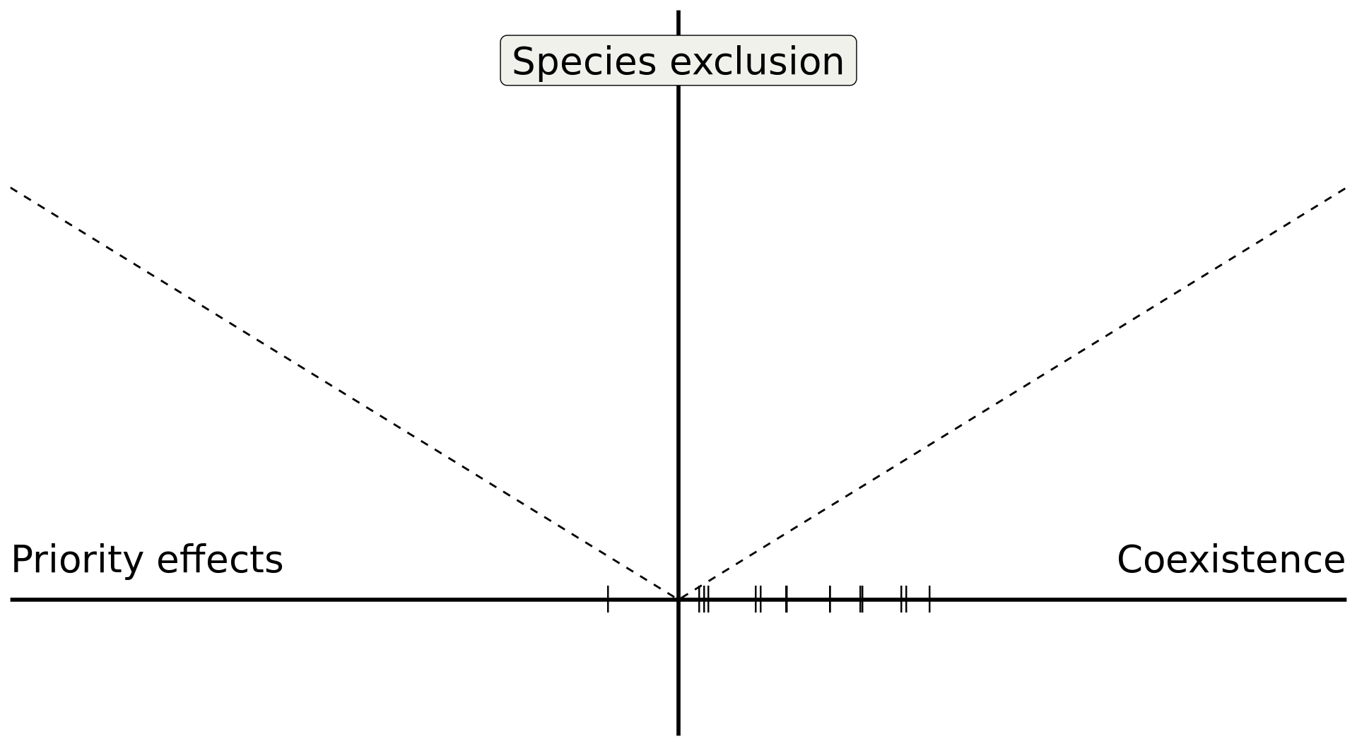
Code
# Example point, using UR_FE values
base_w_rug +
  annotate("pointrange", x = 0.275, y = 0.0591, ymin = 0.0591-0.307,ymax = 0.0591+0.307, shape = 21, stroke = 1.5, size = 1, linewidth = 0.1, fill = "#4477aa") +
    annotate("pointrange", x = 0.275, y = 0.0591, xmin = 0.275-0.152,xmax = 0.275+0.152, shape = 21, fill = "#4477aa", linewidth = 0.1, size = 1, stroke = 1.5) +
annotate("text", x = 0.275 + 0.3, y = 0.0591 + 0.15, color = "#4477aa", label = "Festuca - Plantago", size = 8, fontface = "italic") 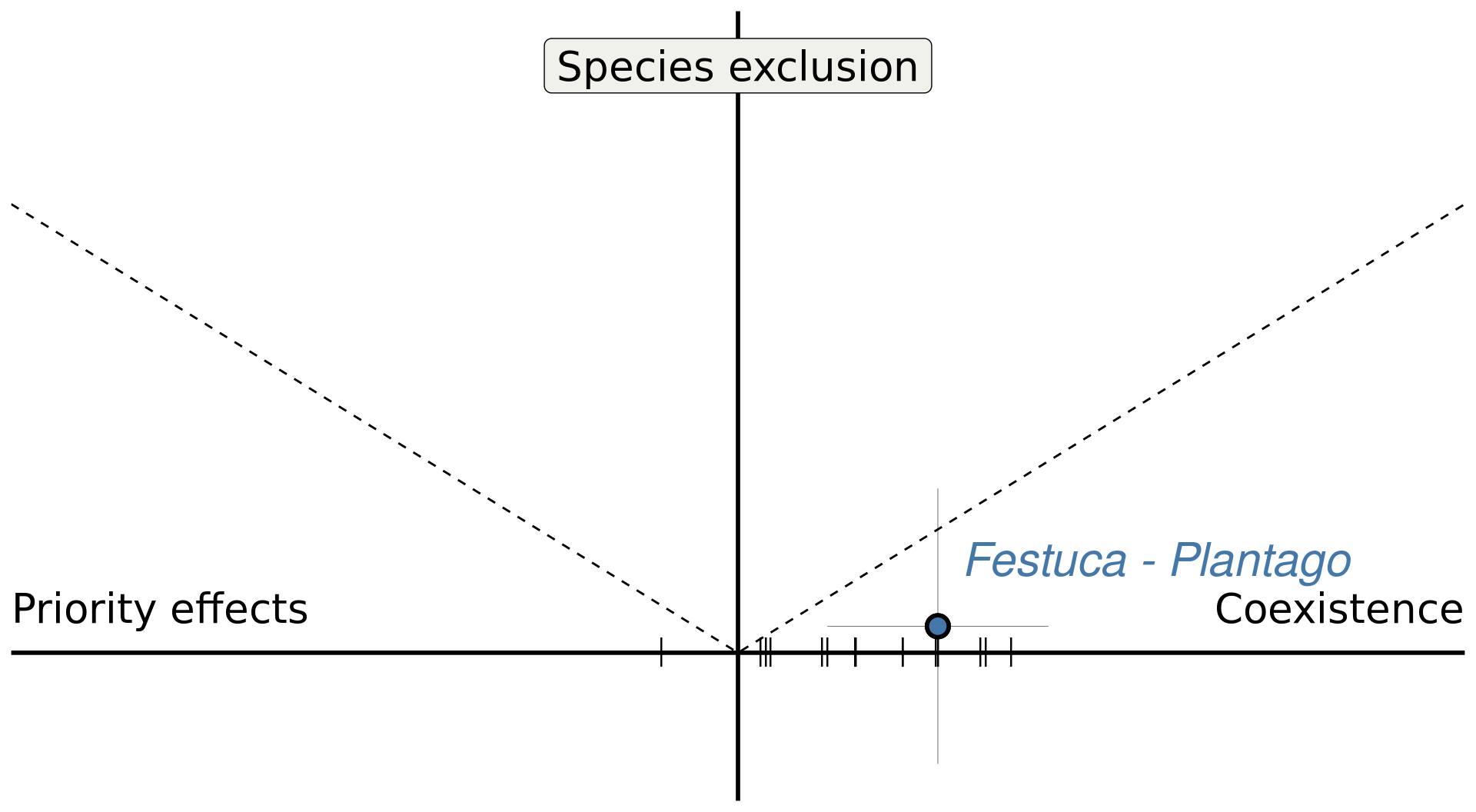
Code
base +
  geom_pointrange(data = sd_fd_summary,
                  aes(x = mean_sd, y = mean_fd,
                      ymin = mean_fd-sem_fd,
                      ymax = mean_fd+sem_fd, fill = outcome2), size = 1, linewidth = 0.1,
                  shape = 21, stroke = 1.5) +
    geom_pointrange(data = sd_fd_summary,
                  aes(x = mean_sd, y = mean_fd,
                      xmin = mean_sd-sem_sd,
                      xmax = mean_sd+sem_sd, fill = outcome2), size = 1,
                  linewidth = 0.1, shape = 21, stroke = 1.5) +
  scale_fill_manual(values = c("#4477aa", "#ee6677", "#ccbb44")) +
  theme(legend.position = "none")+
  theme(axis.title = element_blank())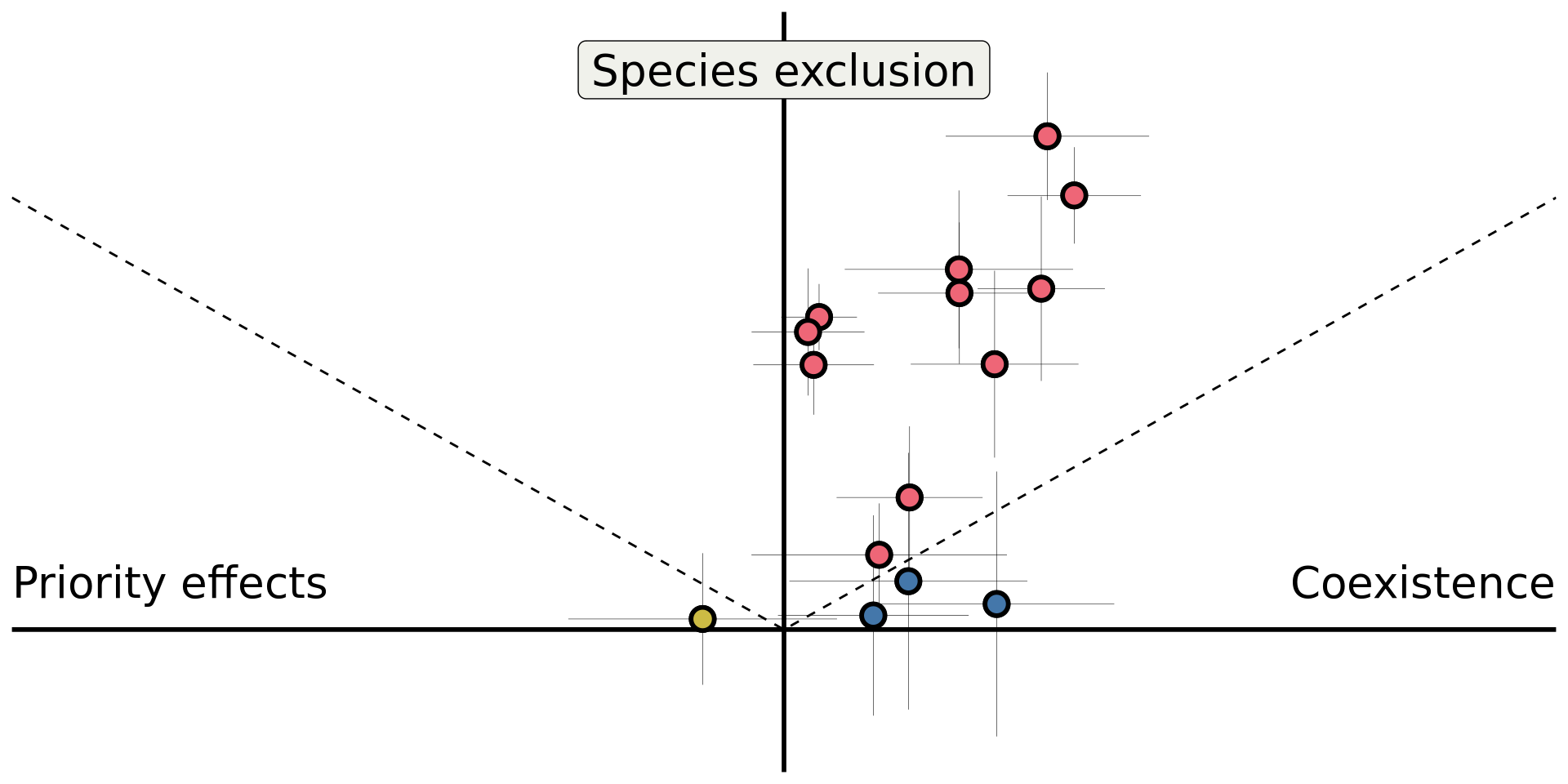
Detailed in Kandlikar et al. (2021)
Do microbes generate fitness differences in nature?
In California grasslands, microbes tend to drive stronger fitness differences than stabilization.
Can we answer this question more generally?


Results in Yan, Levine, and Kandlikar (2022); Analyses available on Zenodo

Microbially-mediated coexistence in pine-oak forests in Spain, Pajares-Murgó et al. (2024)
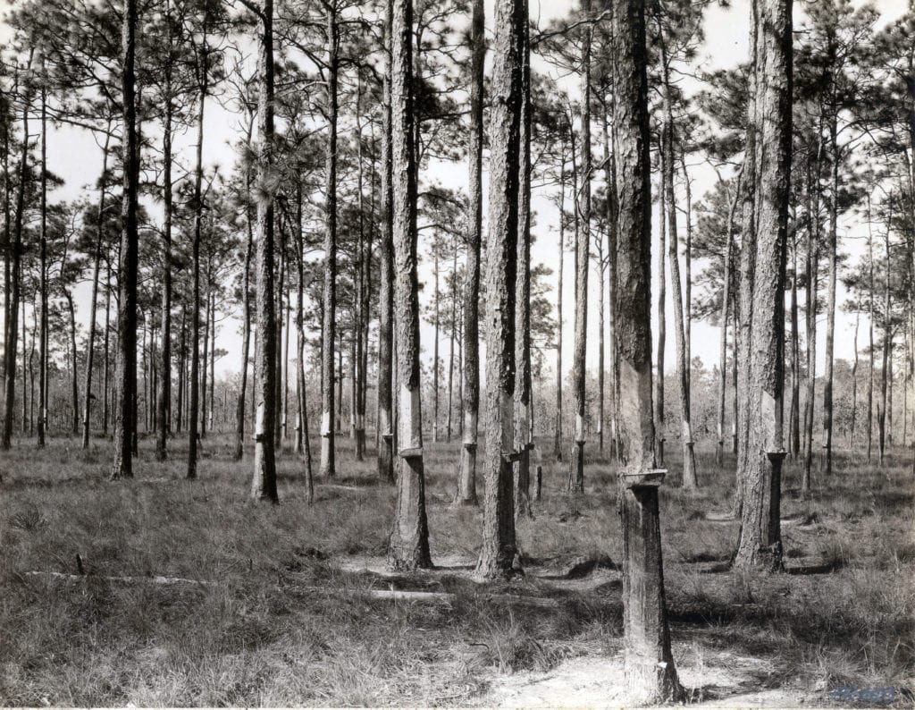
Historical range of the longleaf pine ecosystem
Code
library(sf)
library(tidyverse)

little <- sf::st_read("../img/pinupalu.shp")
## Reading layer `pinupalu' from data source
##   `/home/gkandlikar@lsu.edu/gklab/talks/img/pinupalu.shp' using driver `ESRI Shapefile'
## Simple feature collection with 38 features and 5 fields
## Geometry type: POLYGON
## Dimension:     XY
## Bounding box:  xmin: -95.21806 ymin: 26.61921 xmax: -75.79999 ymax: 36.84856
## CRS:           NA

# States we want to show
llp_states <- c("texas", "louisiana","mississippi", "alabama", "florida", "georgia", "south carolina", "north carolina", "virginia", "tennessee")
states <- map_data("state") |>
  filter(region %in% llp_states)

ggplot() +
  geom_polygon(data = states,
               aes(x = long, y = lat, group = group), fill = "transparent", color = 'darkgrey') +
  geom_sf(data = little, fill = alpha('#228833', 0.5)) +
  theme_void()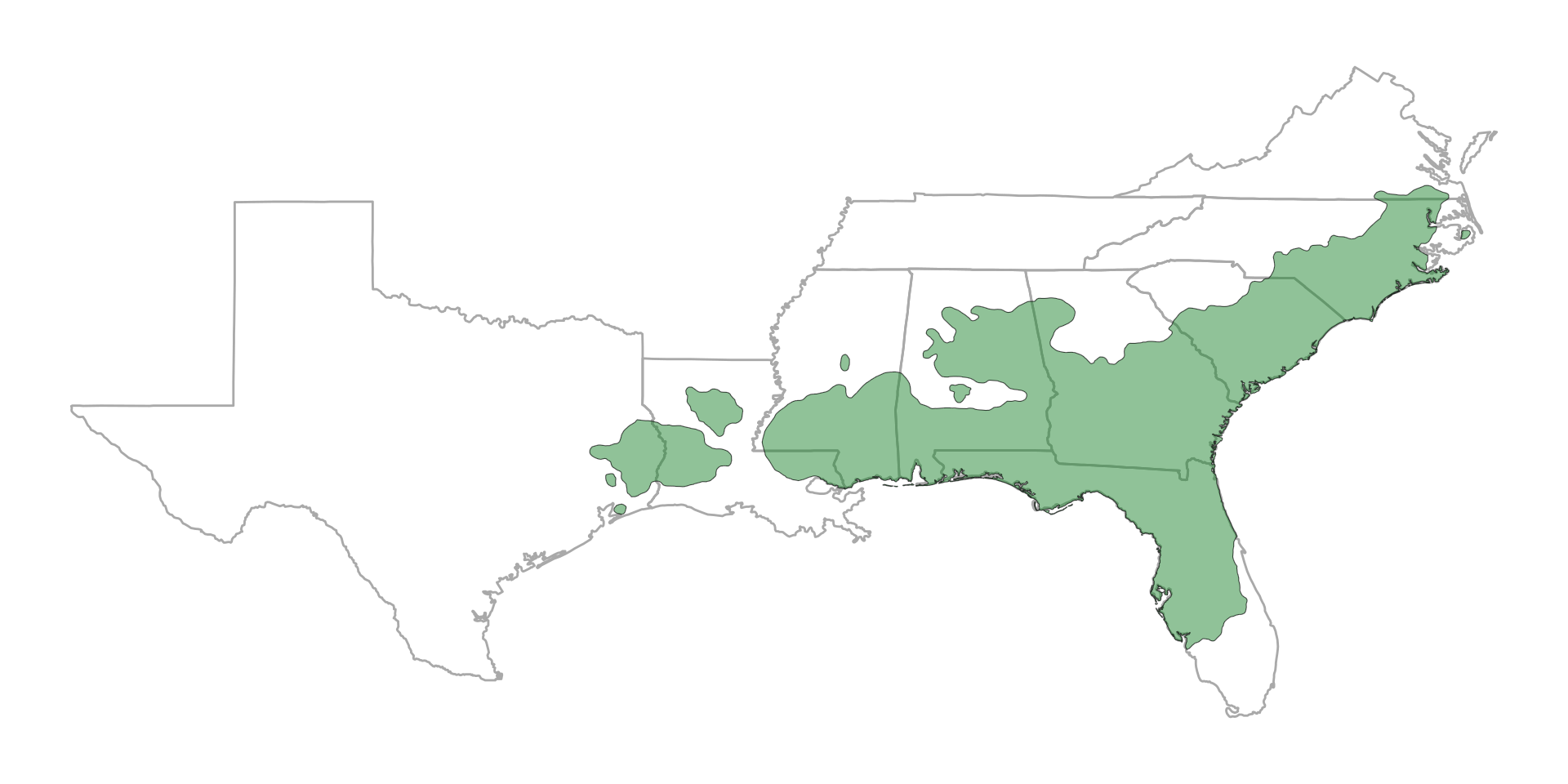
Fire helps maintain the open understory
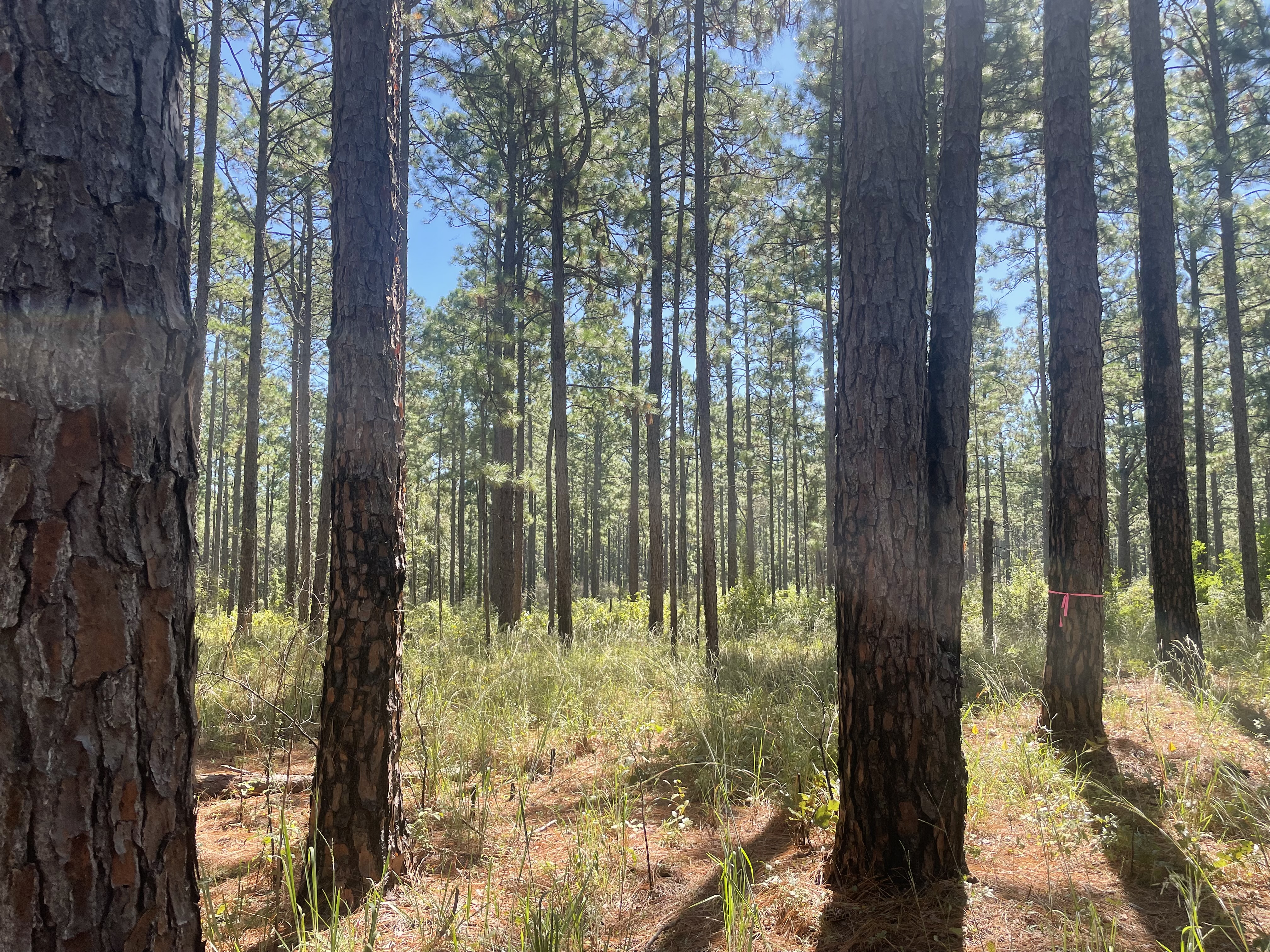
Remarkable diversity at small spatial scales (40-50 plant spp/m2)
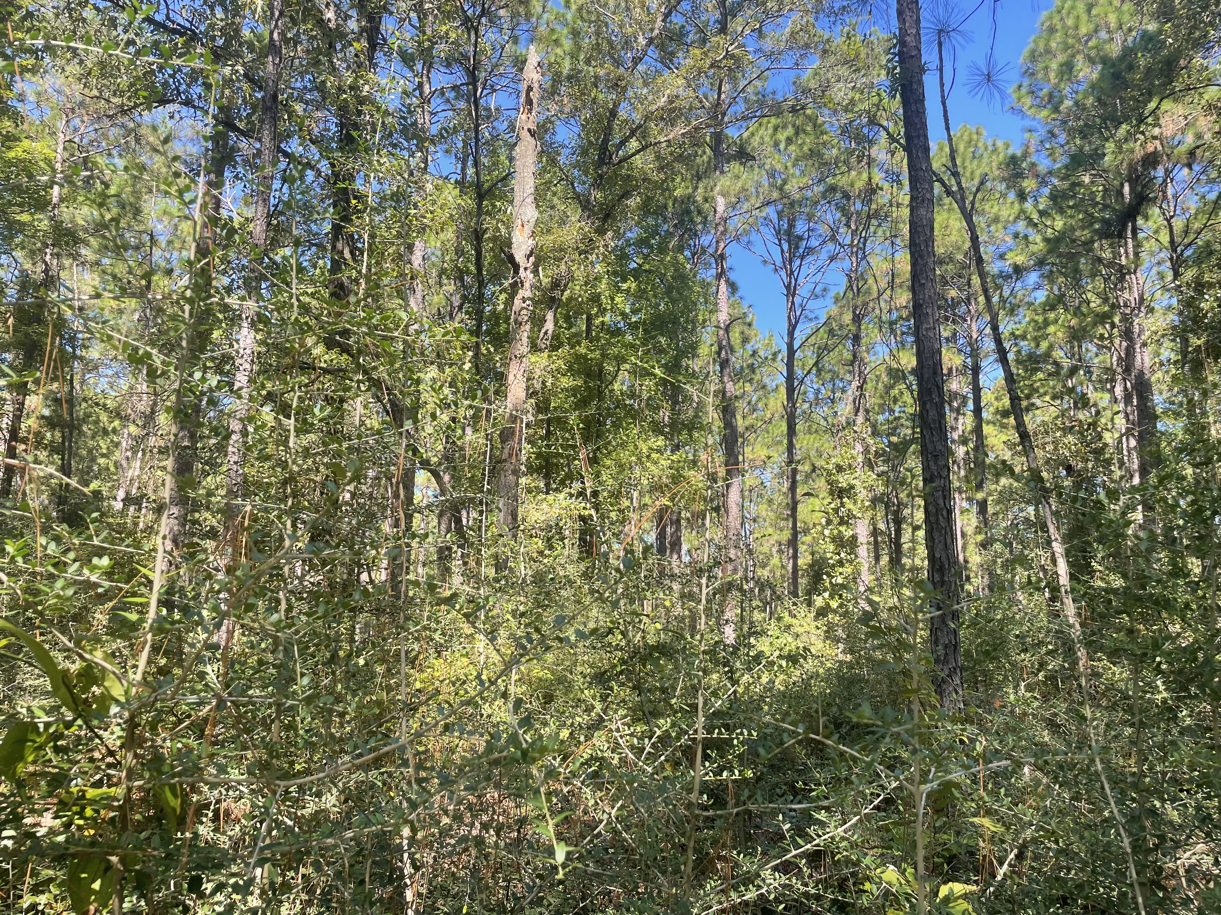
Woody encroachment pervasive under fire suppression
Woody encroachment is common worldwide
Over 500 million hectares of grasslands/savannas affected
Many drivers… but we wonder if there is a role for plant–soil microbial feedbacks.

1. Across ecosystems, grasses tend to grow worse with conspecific-conditioned soil microbes
Code
# curl::curl_download("https://datadryad.org/downloads/file_stream/2789266", destfile = "../data/jiang2024-dataset.csv")

jiang_dat <- read_csv("../data/jiang2024-dataset.csv")


# jiang_metamod  <- metafor::rma.mv(rr, var, data = jiang_dat,   mods = ~ Life.form-1)
# saveRDS(jiang_metamod, "../data/jiang-metamod.rds")

metamod <- readRDS("../data/jiang-metamod.rds")

metamod_s <- broom::tidy(metamod)

jiang_plot <-
jiang_dat |>
  ggplot(aes(x = rr, y = Life.form, color = Life.form)) +
  ggbeeswarm::geom_quasirandom(shape = 21) +
  scale_color_manual(values = c("#ccbb44","transparent")) +
  annotate("point",
           x = metamod_s$estimate[1], y = 1, size = 3, shape = 21, stroke = 1.5) +
  # annotate("point",
  #          x = metamod_s$estimate[2], y = 2, size = 3, shape = 21, stroke = 1.5) +
  ylab("") +
  xlab("Growth in self vs. growth in non-self") +
    xlim(-2.5,2.5)+
  geom_vline(xintercept = 0, linetype = 'dashed') +
  theme(legend.position = "none",
        axis.text.y = element_text(size = 12, color = 'black'))
jiang_plot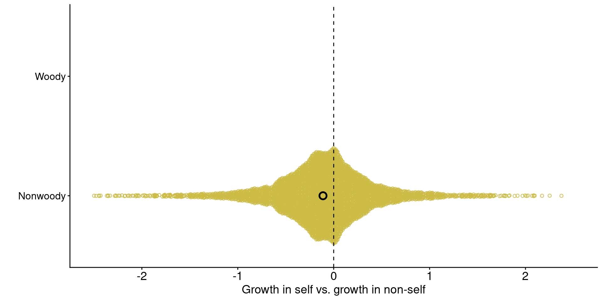
Data from Jiang et al. (2024)
1. Across ecosystems, grasses tend to grow worse with conspecific-conditioned soil microbes
Code
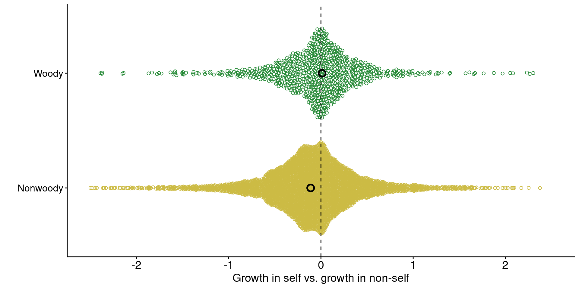
Data from Jiang et al. (2024)
2. Encroaching woody plants often have distinct microbial symbionts.
In African savannas, N-fixing legumes are the primary woody invader in >90% of studies sites (Stevens et al. 2017)
Ectomycorrhizal symbiosis is especially more common among encroaching woody plants (Simha and Kandlikar 2026)
Code
# download.file("https://www.science.org/doi/suppl/10.1126/science.aai8212/suppl_file/bennett_aai8212_database-s1.xlsx", destfile = "../data/bennett2017-dataset.xlsx")
readxl::read_xlsx("../data/bennett-2017.xlsx", sheet = 2) |>
  mutate(`Type of Mycorrhiza` = factor(`Type of Mycorrhiza`, c("EM", "AM"))) |>
  mutate(logratio = log(`Average of Biomass in Conspecific Soil`/`Average of Biomass in Heterospecific Soil`)) |>
  arrange(logratio) |>
  mutate(rown = row_number()) |>
  ggplot(aes(x = logratio, color = `Type of Mycorrhiza`, y = rown, shape = `Type of Mycorrhiza`)) +
  geom_point(size = 2) +
  geom_segment(aes(x = 0, xend = logratio), linewidth = 0.125) +
  xlab("Growth in self-conditioned microbes vs.\n nonself-conditioned microbes") +

  geom_vline(xintercept = 0) +
  scale_color_manual(values = c("#0077bb", "#cc3311")) +
  theme(axis.line.y = element_blank(),
        axis.text.y = element_blank(),
        axis.title.y = element_blank(),
        axis.ticks.y = element_blank(),
        legend.position = "inside",
        legend.position.inside = c(0.9, 0.1),
        legend.text = element_text(size = 12),
        legend.title = element_blank())
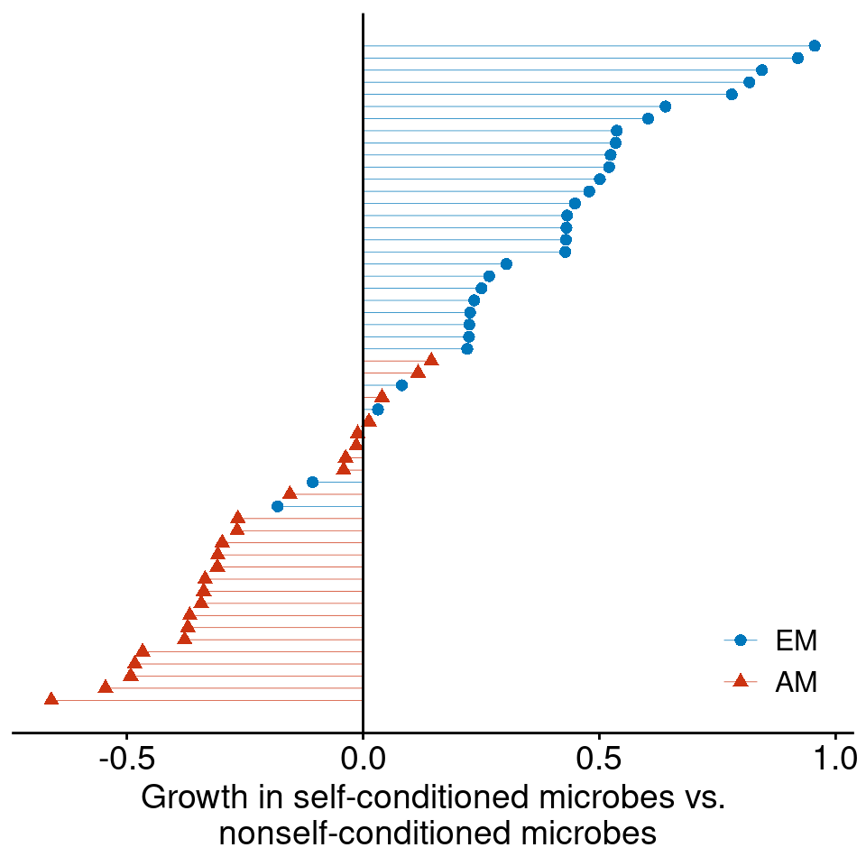
Data from Bennett et al. (2017)
Mathematical modeling of plant dynamics

Model dynamics in the absence of fire
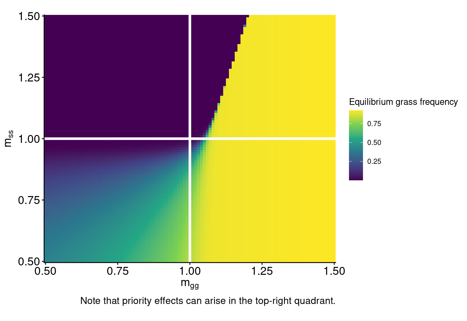
Model dynamics in the absence of fire
Code
library(tidybayes)

meta <- readRDS("../img/swj-brms-meta.RDS")

b_draws <-
  meta |>
  spread_draws(b_Life.formNonwoody, b_Life.formWoody) |>
  rename(mgg_draws = b_Life.formNonwoody,
         mss_draws = b_Life.formWoody) |>
  median_qi() |>
  mutate(across(is.numeric, exp))

plot_det_pt <-
  plot_det +
  geom_pointrange(inherit.aes = F,
                  data = b_draws,
                  aes(x = mgg_draws, y = mss_draws,
                      xmin = mgg_draws.lower, xmax = mgg_draws.upper),
                  color = 'white', shape = 21, size = 1, stroke = 2) +
  geom_pointrange(inherit.aes = F,
                  data = b_draws,
                  aes(x = mgg_draws, y = mss_draws,
                      ymin = mss_draws.lower, ymax = mss_draws.upper),
                  color = 'white', shape = 21,  size = 1, stroke = 2) +
  labs(caption = "White point & error bars show median & 95 CrI of Bayesian meta-analysis\nof grasses and woody plants from areas undergoing encroachment.")
plot_det_pt
How does fire alter microbial regulation of plant communities?

Fires alter plant and microbial states
Fires of higher intensities cause more mortality of grasses, woody seedlings, and soil microbes.
In general, woody plants are more fire-sensitive than grasses, but their sensitivity varies by life stage.
Three scenarios of fire impacts on woody adults:
Code
int = seq(0,1, length.out = 20)
fire = data.frame(int = seq(0,1, length.out = 20),
                  grass = 1/(1+150*exp(-10.02*int)),
                  seedling = 1/(1+150*exp(-20.04*int)),
                  adult = 1/(1+150*exp(-10.02*int)),
                  sens = rep("Fire Sensitive", 20)) |>
  pivot_longer(cols=c(grass,seedling,adult), names_to = "Plant", values_to = "mort")
fire2 = fire |> mutate(sens = "Less Sensitive",
                       mort = case_when(Plant == "adult" ~ mort/2, TRUE ~ mort))
fire3 = fire |> mutate(sens = "Not Sensitive",
                       mort = case_when(Plant == "adult" ~ 0, TRUE ~ mort))

fire_all = rbind(fire, fire2, fire3) |> mutate(sens = as.factor(sens), Plant = as.factor(Plant))
levels(fire_all$sens)
## [1] "Fire Sensitive" "Less Sensitive" "Not Sensitive"
levels(fire_all$Plant) = c("Woody Adult", "Grass", "Woody Seedling")
fire_all$Plant = factor(fire_all$Plant, levels = c("Grass", "Woody Seedling", "Woody Adult"))

scenarios = ggplot(data = fire_all, aes(x = int, y = mort, group = Plant)) +
  geom_path(aes(color = Plant, linetype = Plant), linewidth = 3) +
  scale_color_manual(values = c("#FDE725FF", "#2A788EFF", "#440154FF"))+
  scale_linetype_manual(values = c("solid", "dashed", "longdash"))+
  labs(x = "Fire Intensity", y="Percent Mortality")+
  scale_x_continuous(expand = c(0,0), breaks = c(0.25, 0.5, 0.75, 1.0)) +
  scale_y_continuous(expand = c(0,0))+
  facet_wrap(~ sens)
scenarios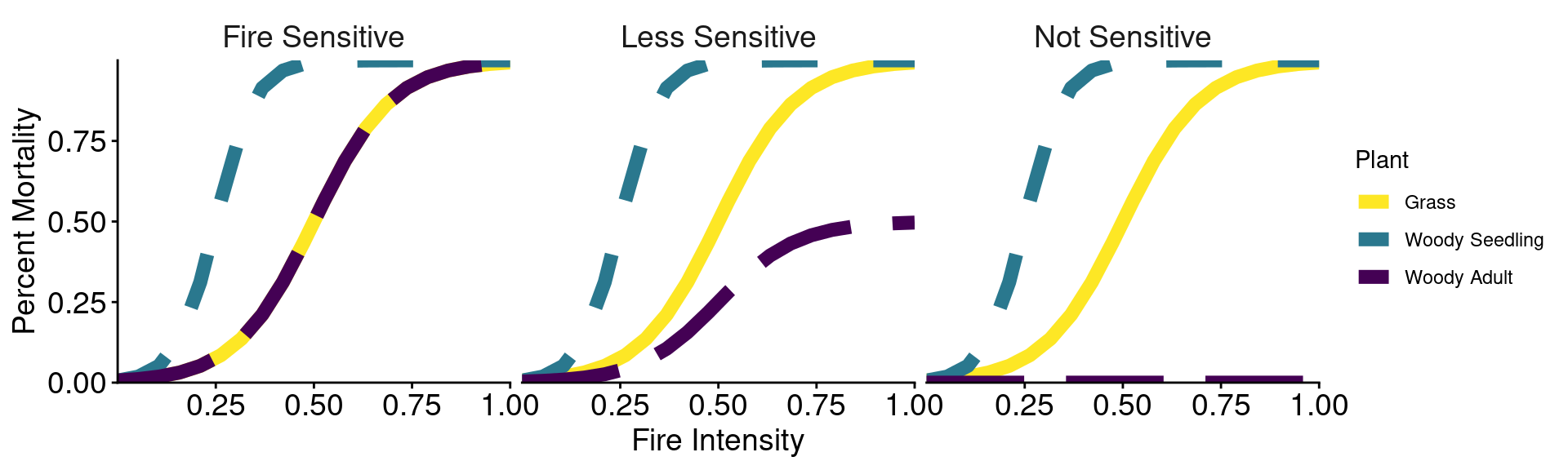
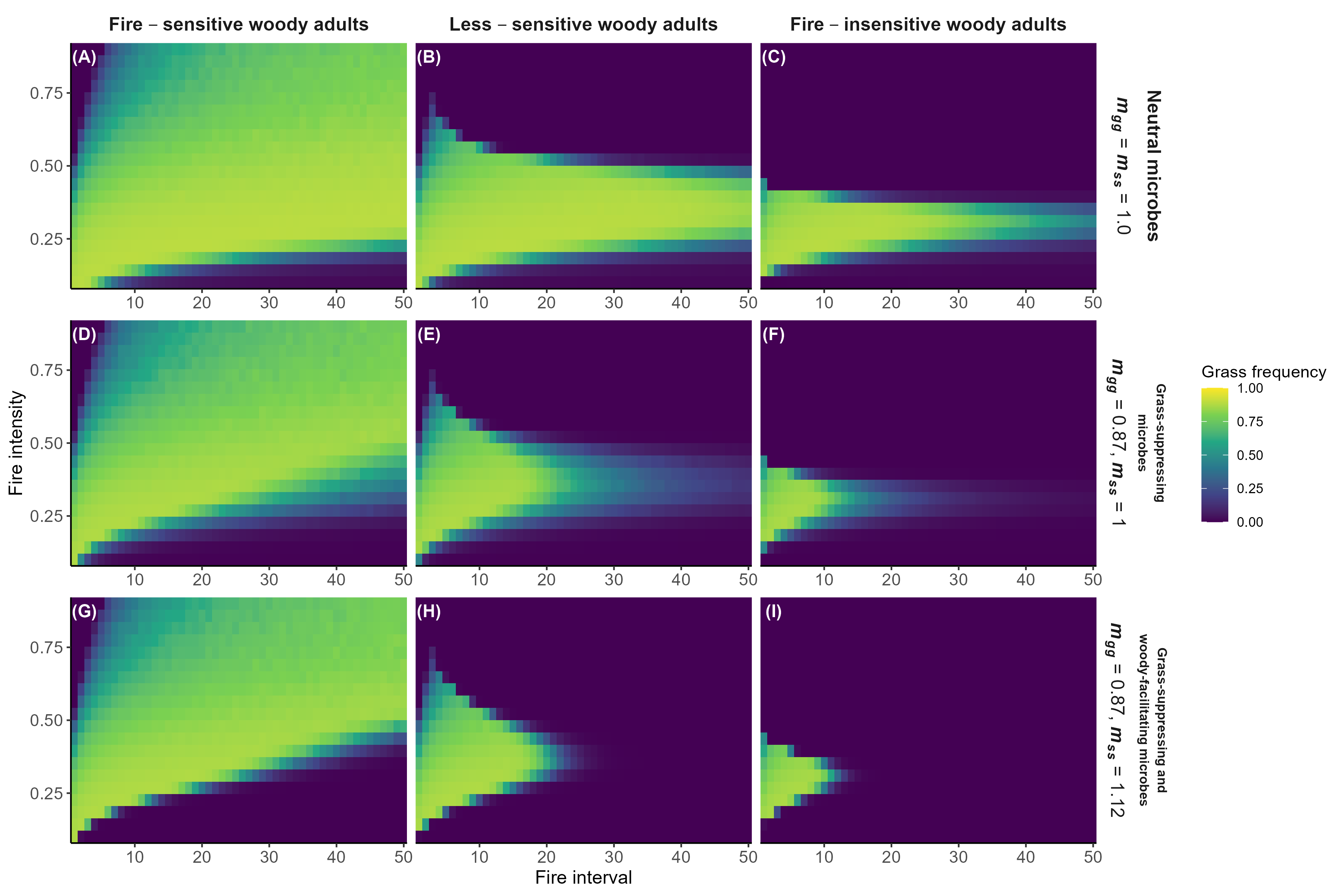
Model predictions with fire
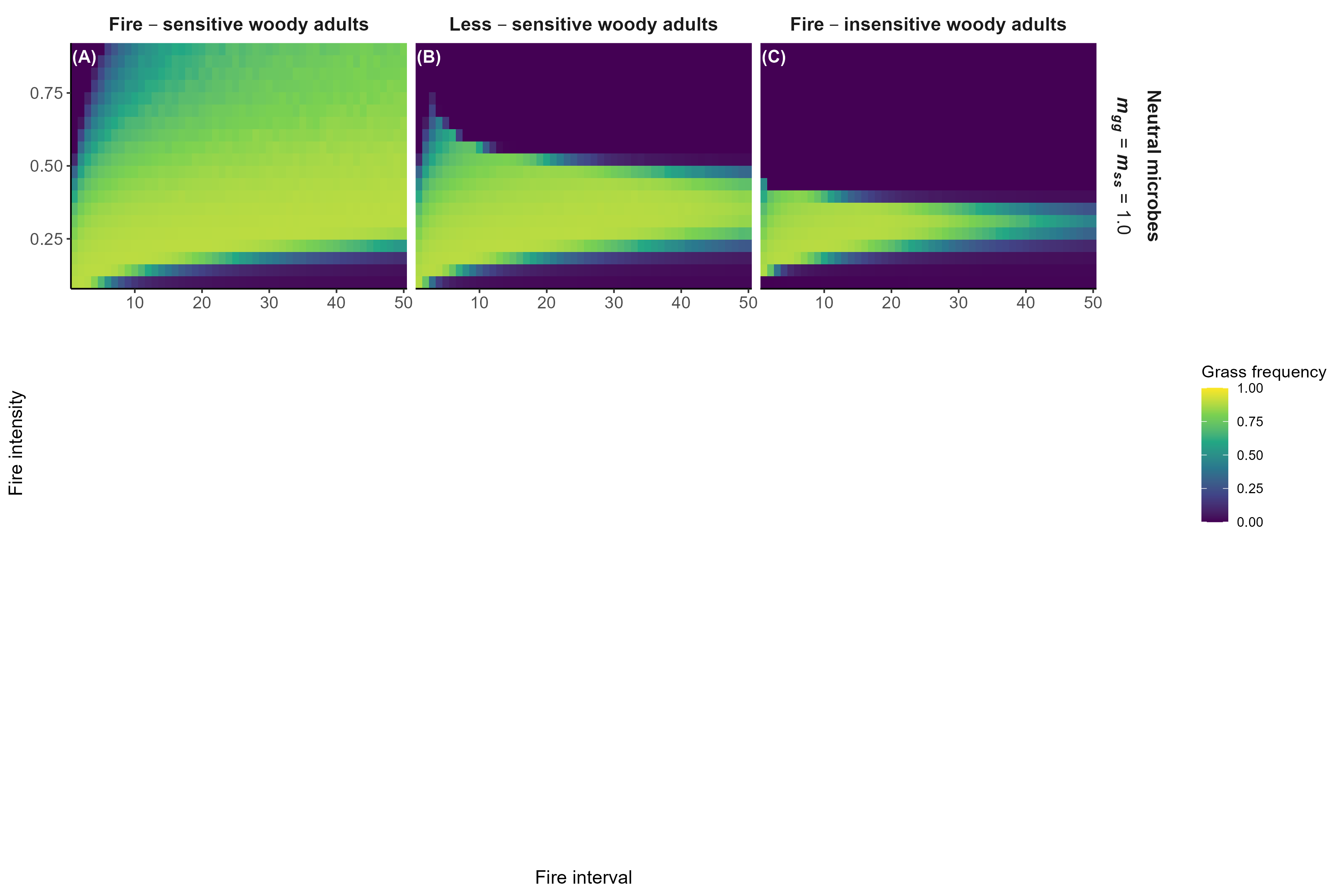
Model predictions with fire
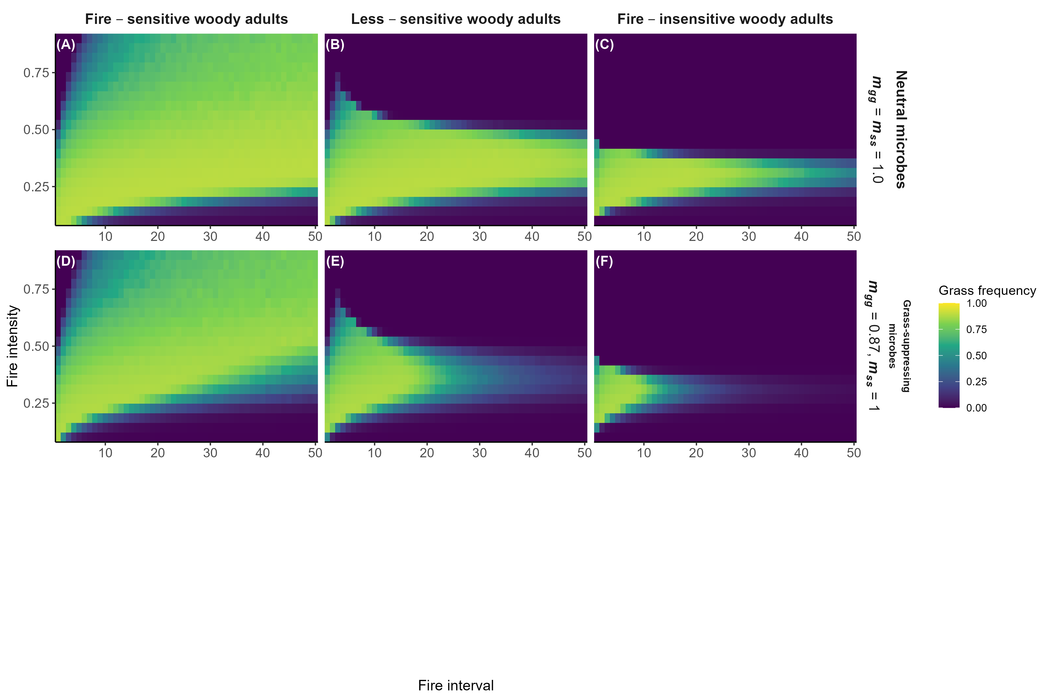
Model predictions with fire
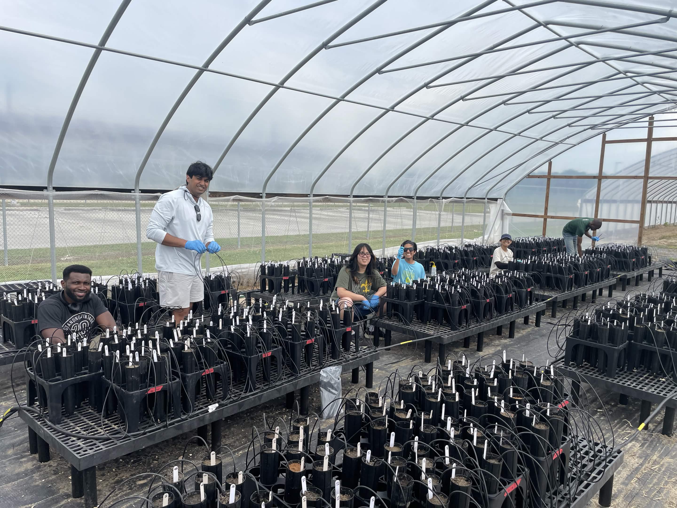
Plant growth experiments to estimate model parameters
Historical perspective on fire in longleaf pine

1. Drought conditions result in a fitness cost.
Code
brapa <-
  read_csv("brapa-data.csv") |>
  pivot_wider(names_from = Type, values_from = y) |>
  mutate(Seed = ifelse(Seed == "HW", "Control", "Low Water"),
         Soil = ifelse(Soil == "HW", "Control", "Low Water"),
         Current = ifelse(Current == "HW", "Control", "Low Water"))
brapa |>
  group_by(Current) |>
  summarize(mean = mean(mean)) |>
  ggplot(aes(x = Current, y = mean)) +
  geom_point(size = 4) +
  ylim(0,250) +
  labs(caption = "Marginal means from a Bayesian GLM (Poisson family)",
       y = "Per-capita fecundity",
       xlab = "")
2. Maternal effects help alleviate fitness cost of drought.

3. Do droughted soils further alleviate drought stress?
Code
brapa |>
  ggplot(aes(x = Current, y = mean, ymin = sdlo, ymax = sdhi,
             color = Soil, shape = Seed)) +
  geom_pointrange(size = 1, position = position_dodge2(width = 0.3)) +
    scale_color_manual(values = c("#4477aa", "#ee6677")) +
    ylim(0,250) +
    labs(caption = "Marginal means & 95% CrIs from a Bayesian GLM (Poisson family)",
         y = "Per-capita fecundity",
         xlab = "")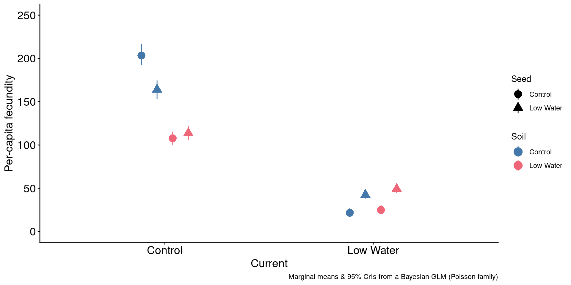
Ongoing efforts to uncover the mechanistic basis.
Focus area 1: Disruptions to plant–soil feedback under habitat fragmentation (Saini et al. accepted at AJB)

Focus area 2: Plant–fungal–nutrient interactions as drivers of monodominance of ectomycorrhizal-associating trees in hyperdiverse forests