Approach
Approach
![]()


Lasting influence of the Bever model
Code
# Dataset downloaded from Figshare:
# curl::curl_download("https://figshare.com/ndownloader/files/14874749", destfile = "../crawford-supplement.xlsx")

read_excel("../data/crawford-supplement.xlsx", sheet = "Data") |>
  mutate(stab = -0.5*rrIs) |> # show in terms of stabilization instead of I_s
  filter(stab > -3) |> # Remove the pair with Stab approx. 6 -- according to McCarthy Neuman (original author), this is likely due to bad seed survival
  ggplot(aes(x = stab)) +
  geom_histogram(color = "black") +
  geom_histogram(fill = "#56A0D3") +
  geom_rug(color = "grey25") +
  geom_vline(xintercept = 0) +
  annotate("text", x = Inf, y = Inf, label = "N = 1037 pairwise comparisons\n
           57% experience positive stabilization",
           vjust=1, hjust = 1, size = 6) +
  xlab("Stabilization") + ylab("Count")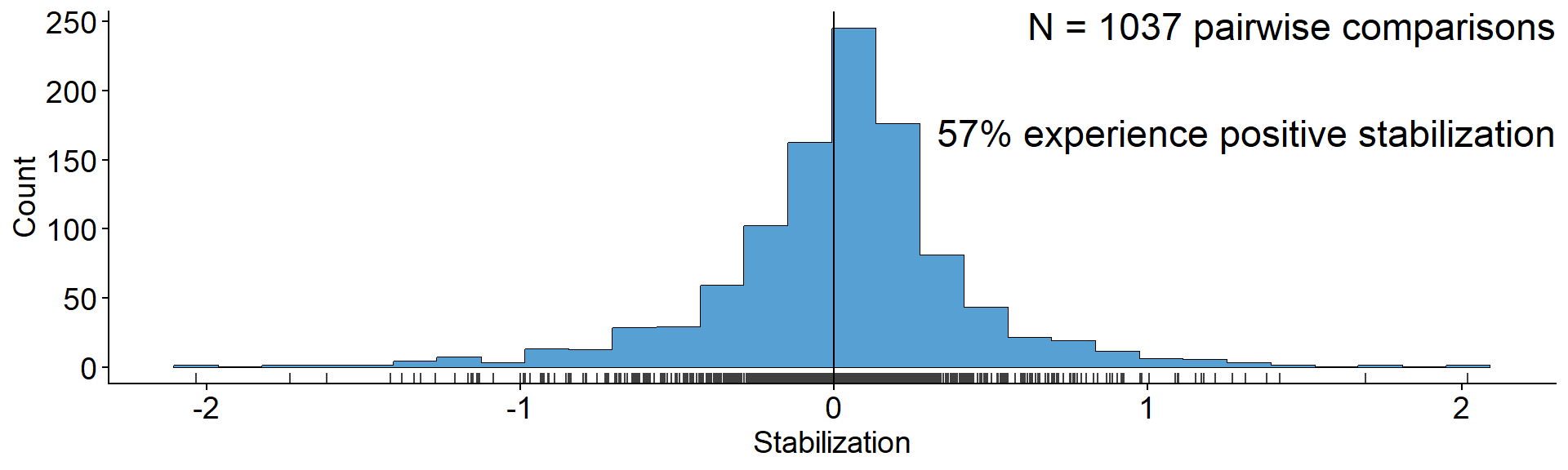
Data from Crawford et al. (2019)
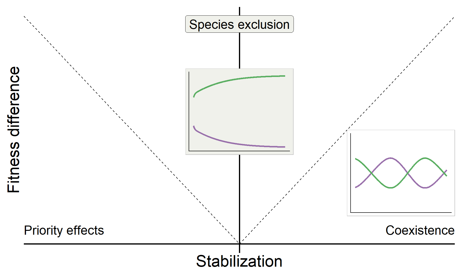
A puzzle: same stabilization, different model dynamics
Code
# Define a function used for making the PSF framework
# schematic, given a set of parameter values
make_params_plot <- function(params, scale = 1.5) {

  color_func <- function(x) {
    ifelse(x < 0, "#EE6677", "#4477AA")
  }
  df <- data.frame(x = c(0,0,1,1),
                   y = c(0,1,0,1),
                   type = c("M", "P", "M", "P"))

  params_plot <-
    ggplot(df) +
    annotate("text", x = 0, y = 1.1, size = 3.25, label = "Plant 1", color = "white", fill = "#9970ab", fontface = "bold") +
    annotate("text", x = 1, y = 1.1, size = 3.25, label = "Plant 2", color = "white", fill = "#5aae61", fontface = "bold") +
    annotate("text", x = 0, y = -0.15, size = 3.25, label = "Soil\nmicrobes A", label.size = 0, fill = "transparent") +
    annotate("text", x = 1, y = -0.15, size = 3.25, label = "Soil\nmicrobes B", label.size = 0, fill = "transparent") +
    annotate("text", x = 0.45, y = -0.4, size = 3.5, fill = "transparent",
               label.size = 0.05,
               label = (paste0("Stabilization = ",
                                  0.5*(params["m1B"] + params["m2A"] - params["m1A"] - params["m2B"])))) +
    geom_segment(aes(x = 0, xend = 0, y = 0.1, yend = 0.9),
                 arrow = arrow(length = unit(0.03, "npc")),
                 linewidth = abs(params["m1A"])*scale,
                 color = alpha(color_func(params["m1A"]), 1)) +
    geom_segment(aes(x = 0.05, xend = 0.95, y = 0.1, yend = 0.9),
                 arrow = arrow(length = unit(0.03, "npc")),
                 linewidth = abs(params["m2A"])*scale,
                 color = alpha(color_func(params["m1B"]),1)) +
    geom_segment(aes(x = 0.95, xend = 0.05, y = 0.1, yend = 0.9),
                 arrow = arrow(length = unit(0.03, "npc")),
                 linewidth = abs(params["m1B"])*scale,
                 color = alpha(color_func(params["m2A"]), 1)) +
    geom_segment(aes(x = 1, xend = 1, y = 0.1, yend = 0.9),
                 arrow = arrow(length = unit(0.03, "npc"),),
                 linewidth = abs(params["m2B"])*scale,
                 color = alpha(color_func(params["m2B"]), 1)) +

    # Plant cultivation of microbes
    geom_segment(aes(x = -0.25, xend = -0.25, y = 0.9, yend = 0.1), linewidth = 0.15, linetype = 1,
                 arrow = arrow(length = unit(0.03, "npc"))) +
    geom_segment(aes(x = 1.25, xend = 1.25, y = 0.9, yend = 0.1), linewidth = 0.15, linetype = 1,
                 arrow = arrow(length = unit(0.03, "npc"))) +

    annotate("text", x = 0, y = 0.5,
             label = (paste0("m1A = ", params["m1A"])),
             angle = 90, vjust = -0.25, size = 3) +
    annotate("text", x = 1.15, y = 0.5,
             label = (paste0("m2B = ", params["m2B"])),
             angle = -90, vjust = 1.5, size = 3) +
    annotate("text", x = 0.75, y = 0.75,
             label = (paste0("m2A = ", params["m2A"])),
             angle = 45, vjust = -0.25, size = 3) +
    annotate("text", x = 0.25, y = 0.75,
             label = (paste0("m1B = ", params["m1B"])),
             angle = -45, vjust = -0.25, size = 3) +
    xlim(c(-0.4, 1.4)) +
    coord_cartesian(ylim = c(-0.25, 1.15), clip = "off") +
    theme_void() +
    theme(legend.position = "none",
          plot.caption = element_text(hjust = 0.5, size = 10))
  return(params_plot)
}

# Define a function for simulating the dynamics of the
# PSF model with deSolve
params_coex <- c(m10 = 0.16, m20 = 0.16,
                 m1A = 0.11, m1B = 0.26,
                 m2A = 0.27, m2B = 0.13, v = 1)

time <- seq(0,50,0.1)
init_pA_05 <- c(N1 = 3, N2 = 7, p1 = 0.3, pA = 0.3)
out_pA_05 <- ode(y = init_pA_05, times = time, func = psf_model, parms = params_coex) |> data.frame()


params_to_plot_coex <- c(m1A = unname(params_coex["m1A"]-params_coex["m10"]),
                    m1B = unname(params_coex["m1B"]-params_coex["m10"]),
                    m2A = unname(params_coex["m2A"]-params_coex["m20"]),
                    m2B = unname(params_coex["m2B"]-params_coex["m20"]), v=1)
param_plot_coex <-
  make_params_plot(params_to_plot_coex, scale = 6) +
  annotate("text", x = 1.375, y = 0.5,
           label = paste0("v = ", params_coex["v"]),
           angle = -90, vjust = 1.5, size = 3)

panel_abund_coex <-
  out_pA_05 |>
  as_tibble() |>
  select(time, N1, N2) |>
  pivot_longer(N1:N2) |>
  ggplot(aes(x = time, y = value, color = name)) +
  geom_line(linewidth = 0.9) +
  scale_color_manual(values = c("#9970ab", "#5aae61"),
                     name = "Plant species", label = c("Plant 1", "Plant 2"), guide = "none") +
  scale_y_continuous(breaks = c(2e4, 4e4, 6e4, 8e4), labels = scales::scientific) +
  ylab("Abundance") +
  theme(axis.title = element_text(size = 10))

# Panel D: plot for frequencies of both plants when growing
# in dynamic soils
panel_freq_coex <-
  out_pA_05 |>
  as_tibble() |>
  mutate(p2 = 1-p1) |>
  select(time, p1, p2) |>
  pivot_longer(p1:p2) |>
  ggplot(aes(x = time, y = value, color = name)) +
  geom_line(linewidth = 1.2) +
  scale_color_manual(values = c("#9970ab", "#5aae61"),
                     name = "Plant species", label = c("Plant 1", "Plant 2")) +
  scale_y_continuous(limits = c(0,1), breaks = c(0, 0.5, 1)) +
  ylab("Frequency") +
  theme(axis.title = element_text(size = 10))

param_plot_coex +  {panel_abund_coex+panel_freq_coex &
  theme(axis.text = element_text(size = 8), legend.position = 'none')} +
  plot_layout(widths = c(1/3, 2/3))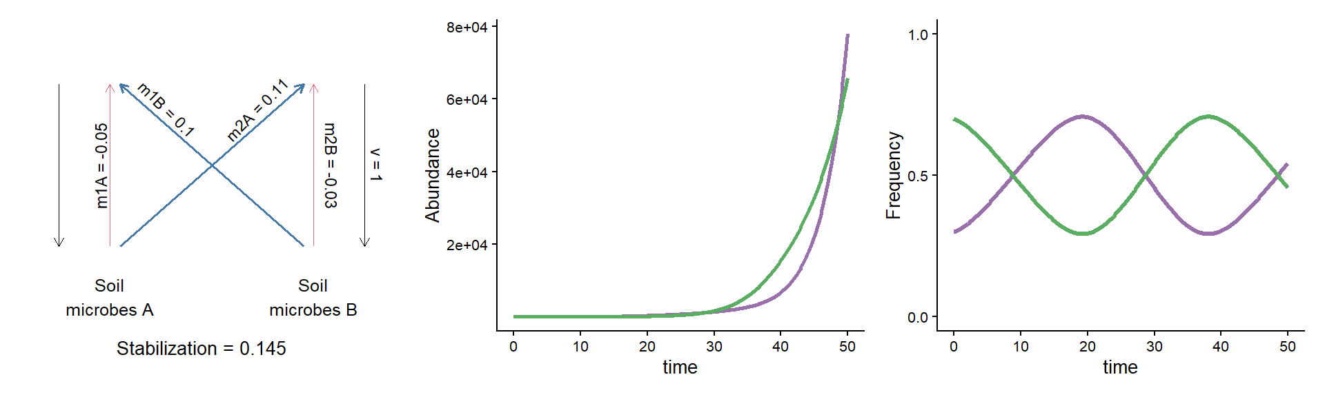
Code
# Define a function for simulating the dynamics of the
# PSF model with deSolve
params <- c(m10 = 0.16, m20 = 0.16,
              m1A = 0.02, m2A = 0.33,
              m1B = 0.18, m2B = 0.20, v = 1)

time <- seq(0,200,0.1)
init_pA_05 <- c(N1 = 3, N2 = 7, p1 = 0.3, pA = 0.3)
out_pA_05 <- ode(y = init_pA_05, times = time, func = psf_model, parms = params) |> data.frame()


params_to_plot <- c(m1A = unname(params["m1A"]-params["m10"]),
                    m1B = unname(params["m1B"]-params["m10"]),
                    m2A = unname(params["m2A"]-params["m20"]),
                    m2B = unname(params["m2B"]-params["m20"]), v=1)
param_plot <-
  make_params_plot(params_to_plot, scale = 6) +
  annotate("text", x = 1.375, y = 0.5,
           label = paste0("v = ", params["v"]),
           angle = -90, vjust = 1.5, size = 3)

panel_abund <-
  out_pA_05 |>
  as_tibble() |>
  select(time, N1, N2) |>
  pivot_longer(N1:N2) |>
  ggplot(aes(x = time, y = value, color = name)) +
  geom_line(linewidth = 0.9) +
  scale_color_manual(values = c("#9970ab", "#5aae61"),
                     name = "Plant species", label = c("Plant 1", "Plant 2"), guide = "none") +
    scale_y_continuous(breaks = c(0,8e17,1.6e18), labels = c("0", "7e17","1.4e18")) +
  ylab("Abundance")

# Panel D: plot for frequencies of both plants when growing
# in dynamic soils
panel_freq <-
  out_pA_05 |>
  as_tibble() |>
  mutate(p2 = 1-p1) |>
  select(time, p1, p2) |>
  pivot_longer(p1:p2) |>
  ggplot(aes(x = time, y = value, color = name)) +
  geom_line(linewidth = 1.2) +
  scale_color_manual(values = c("#9970ab", "#5aae61"),
                     name = "Plant species", label = c("Plant 1", "Plant 2")) +
  scale_y_continuous(limits = c(0,1), breaks = c(0, 0.5, 1)) +
  ylab("Frequency")

param_plot + {panel_abund + panel_freq &
  theme(axis.text = element_text(size = 8), legend.position = 'none')} +
  plot_layout(widths = c(1/3, 2/3))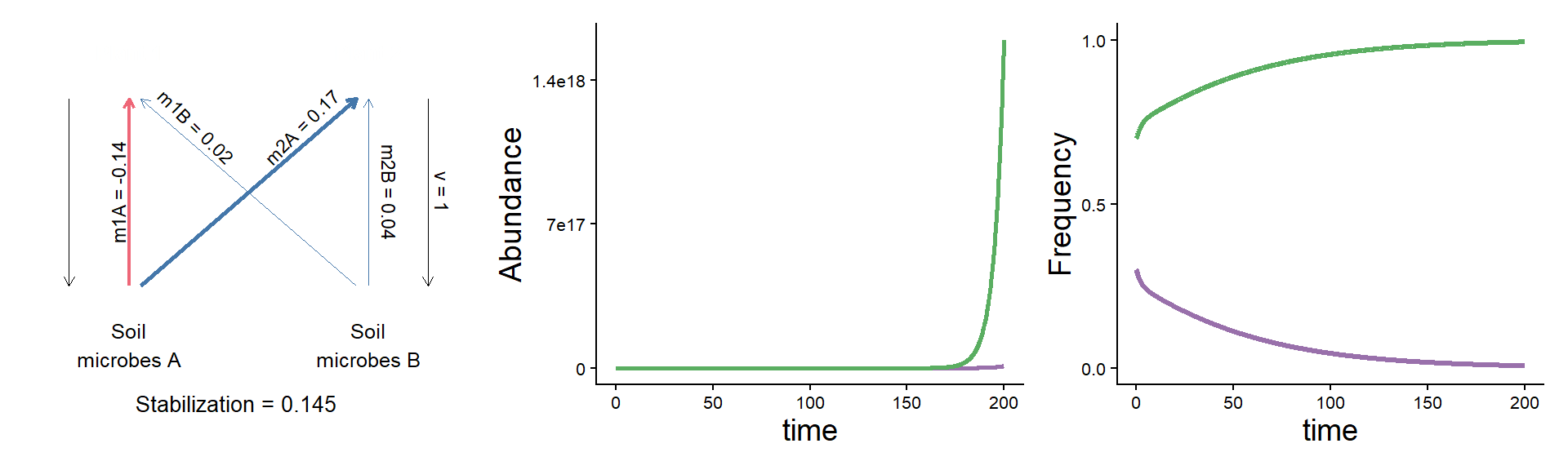
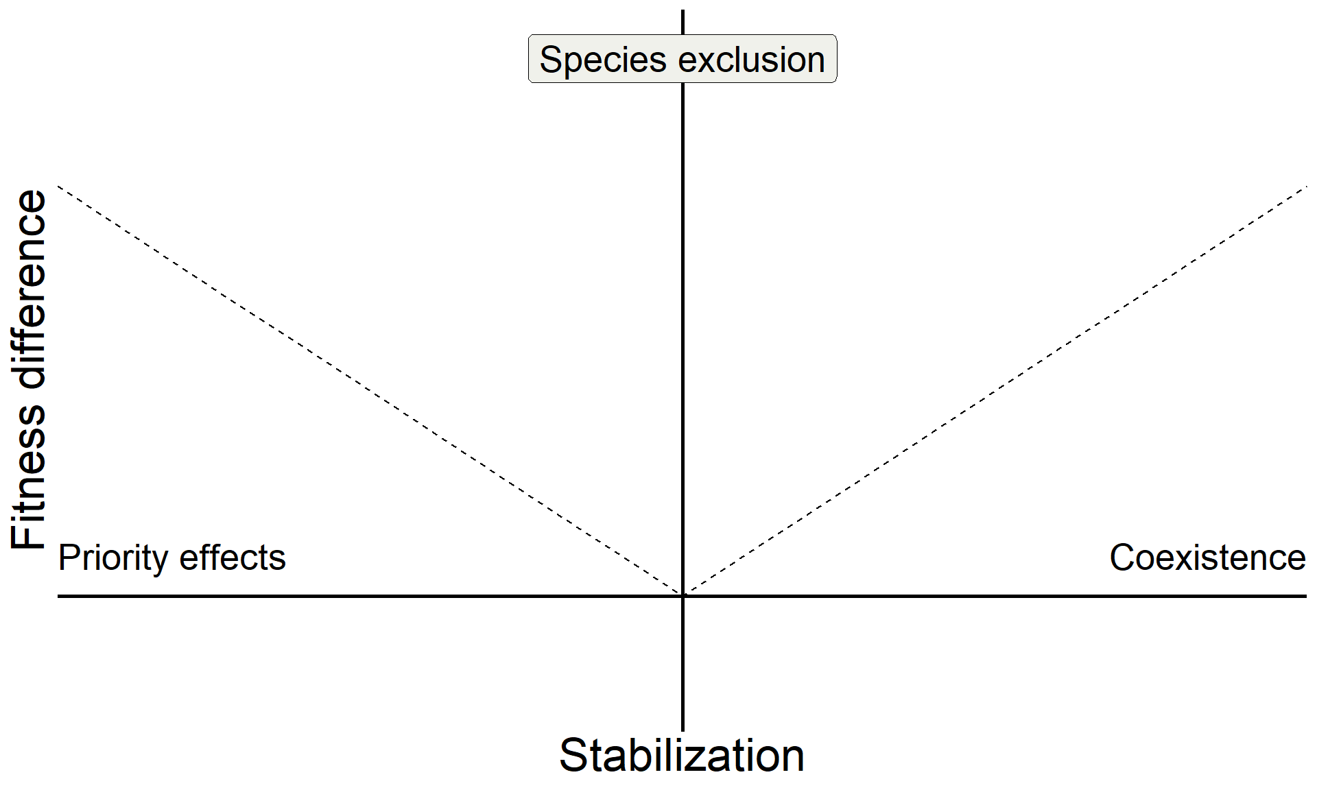
How can we more accurately infer predicted plant dynamics under plant–soil feedback?
Build on insights from coexistence theory (Chesson 2018):
- Stablization is necessary for coexistence but doesn’t guarantee coexistence
- Stable coexistence is possible only when stabilization overcomes competitive imbalances (fitness differences)

How can we more accurately infer predicted plant dynamics under plant–soil feedback?

How can we more accurately infer predicted plant dynamics under plant–soil feedback?
How can we more accurately infer predicted plant dynamics under plant–soil feedback?

How can we more accurately infer predicted plant dynamics under plant–soil feedback?


Code
base <-
  tibble(sd = seq(-1,1,0.1),
       fd = c(seq(1,0,-0.1), seq(0.1,1,0.1))) |>
  ggplot(aes(x = sd, y = fd)) +
  geom_line(linetype = "dashed") +
  geom_hline(yintercept = 0, linewidth = 1) +
  geom_vline(xintercept = 0, linewidth = 1) +
  xlab("Stabilization") +
  ylab("Fitness difference") +
  theme(axis.text = element_blank(),
        axis.ticks = element_blank(),
        axis.line = element_blank(),
        axis.title = element_text(size = 25)) +
  scale_x_continuous(expand = c(0,0)) +
  scale_y_continuous(expand = c(0.04,0))
base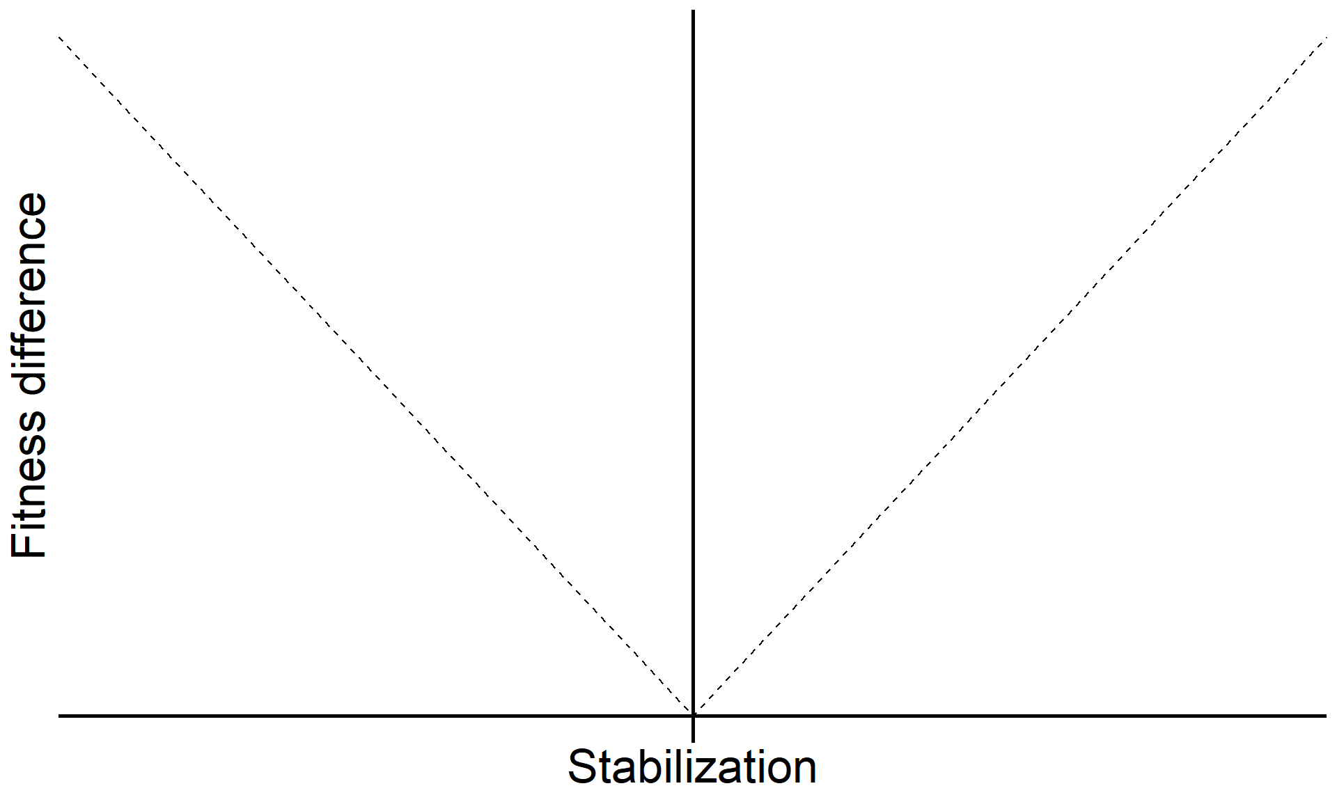
Code
base <-
base +
  annotate("text", x = Inf, y = 0, hjust = 1, vjust = -1, label = "Coexistence", size = 7, family = "italic") +
  annotate("text", x = -Inf, y = 0, hjust = 0, vjust = -1, label = "Priority effects", size = 7, family = "italic") +
  annotate("label", x = 0, y = Inf,  vjust = 1.5, label = "Species exclusion", size = 7, fill = "#F0F1EB",family = "italic")

base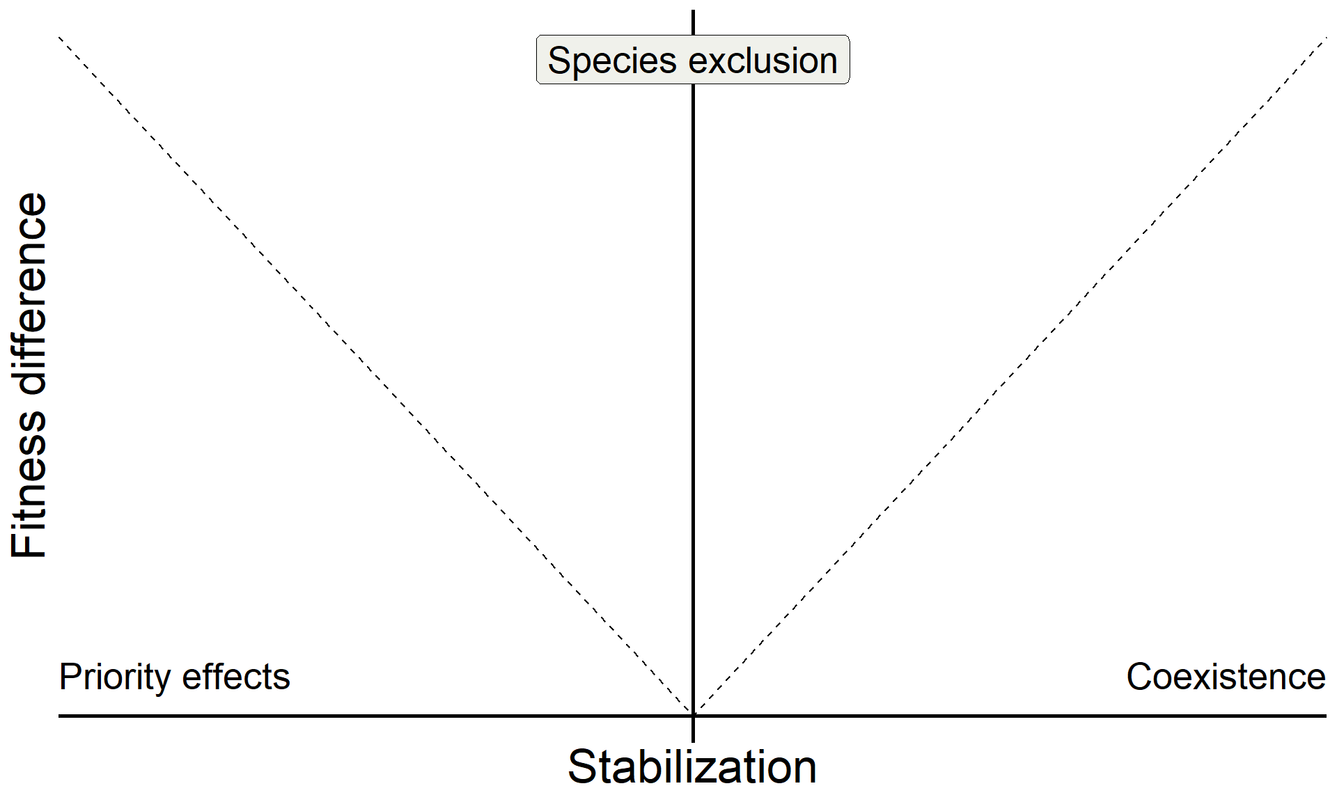
Code
metrics <- function(params) {
  IS <- with(as.list(params), {m1A - m2A - m1B + m2B})
  FD <- with(as.list(params), {(1/2)*(m1A+m2A) - (1/2)*(m1B+m2B)})
  SD <- (-1/2)*IS
  return(c(IS = IS, SD = SD, FD = FD))
}

coex_metrics <- metrics(params_coex)
base_coex <-
  base +
  inset_element({panel_freq_coex + theme(legend.position = 'none',
                                         axis.text = element_blank(),
                                         axis.ticks = element_blank(),
                                         axis.title = element_blank(),
                                         plot.background = element_rect(color = "grey"))},
                0.75,0.15,1,0.5)
base_coex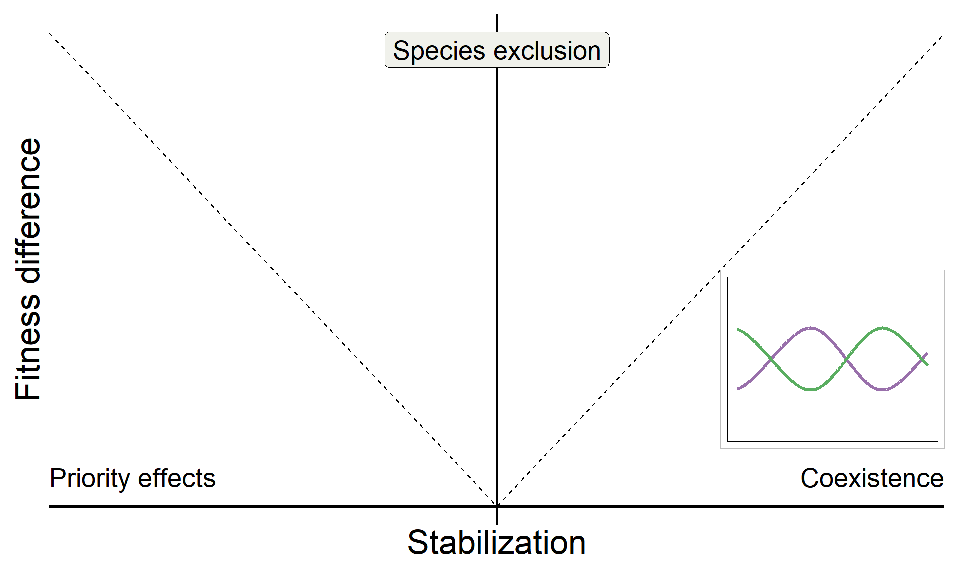


Code
# Example point, using UR_FE values
base +
  annotate("pointrange", x = 0.275, y = 0.0591, ymin = 0.0591-0.307,ymax = 0.0591+0.307, shape = 21, stroke = 1.5, size = 1, linewidth = 0.1, fill = "#4477aa") +
    annotate("pointrange", x = 0.275, y = 0.0591, xmin = 0.275-0.152,xmax = 0.275+0.152, shape = 21, fill = "#4477aa", linewidth = 0.1, size = 1, stroke = 1.5) +
    annotate("text", x = 0.275 + 0.3, y = 0.0591 + 0.15, color = "#4477aa", label = "Festuca - Plantago", size = 8, fontface = "italic") +
  theme(axis.title = element_blank())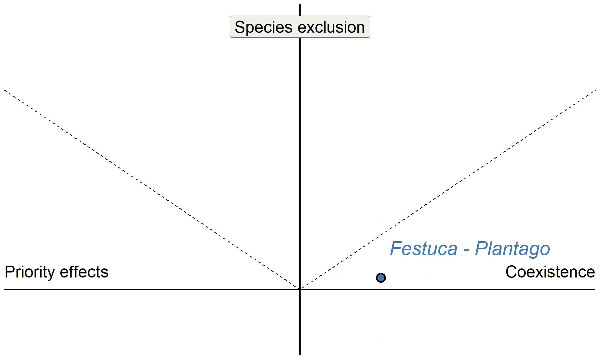
Code
# Dataset downloaded from Figshare:
# curl::curl_download("https://datadryad.org/downloads/file_stream/367188", destfile = "../data/kandlikar2021-supplement.csv")

biomass_wide <-
  read_csv("../data/kandlikar2021-supplement.csv") |>
  mutate(log_agb = log(abg_dry_g)) |>
  mutate(source_soil = ifelse(source_soil == "aastr", "str", source_soil),
                source_soil = ifelse(source_soil == "abfld", "fld", source_soil),
                pair = paste0(source_soil, "_", focal_species)) |>
      select(replicate, pair, log_agb)  |>
    pivot_wider(names_from = pair, values_from = log_agb) |>
  filter(!is.na(replicate))

# Calculate the Stabilization between each species pair ----
# Recall that following the definition of the m terms in Bever 1997,
# and the analysis of this model in Kandlikar 2019,
# stablization = -0.5*(log(m1A) + log(m2B) - log(m1B) - log(m2A))
# Here is a function that does this calculation
# (recall that after the data reshaping above,
# each column represents a given value of log(m1A))
calculate_stabilization <- function(df) {
  df |>
    # In df, each row is one repilcate/rack, and each column
    # represents the growth of one species in one soil type.
    # e.g. "FE_ACWR" is the growth of FE in ACWR-cultivated soil.
    mutate(AC_FE = -0.5*(AC_ACWR - AC_FEMI - FE_ACWR + FE_FEMI),
           AC_HO = -0.5*(AC_ACWR - AC_HOMU - HO_ACWR + HO_HOMU),
           AC_SA = -0.5*(AC_ACWR - AC_SACO - SA_ACWR + SA_SACO),
           AC_PL = -0.5*(AC_ACWR - AC_PLER - PL_ACWR + PL_PLER),
           AC_UR = -0.5*(AC_ACWR - AC_URLI - UR_ACWR + UR_URLI),
           FE_HO = -0.5*(FE_FEMI - FE_HOMU - HO_FEMI + HO_HOMU),
           FE_SA = -0.5*(FE_FEMI - FE_SACO - SA_FEMI + SA_SACO),
           FE_PL = -0.5*(FE_FEMI - FE_PLER - PL_FEMI + PL_PLER),
           FE_UR = -0.5*(FE_FEMI - FE_URLI - UR_FEMI + UR_URLI),
           HO_PL = -0.5*(HO_HOMU - HO_PLER - PL_HOMU + PL_PLER),
           HO_SA = -0.5*(HO_HOMU - HO_SACO - SA_HOMU + SA_SACO),
           HO_UR = -0.5*(HO_HOMU - HO_URLI - UR_HOMU + UR_URLI),
           SA_PL = -0.5*(SA_SACO - SA_PLER - PL_SACO + PL_PLER),
           SA_UR = -0.5*(SA_SACO - SA_URLI - UR_SACO + UR_URLI),
           PL_UR = -0.5*(PL_PLER - PL_URLI - UR_PLER + UR_URLI)) |>
    select(replicate, AC_FE:PL_UR) |>
    gather(pair, stabilization, AC_FE:PL_UR)
}

stabilization_values <- calculate_stabilization(biomass_wide)
# Seven values are NA; we can omit these
stabilization_values <- stabilization_values |>
  filter(!(is.na(stabilization)))

# Calculating the Fitness difference between each species pair ----
# Similarly, we can now calculate the fitness difference between
# each pair. Recall that FD = 0.5*(log(m1A)+log(m1B)-log(m2A)-log(m2B))
# But recall that here, IT IS IMPORTANT THAT
# m1A = (m1_soilA - m1_fieldSoil)!

# The following function does this calculation:
calculate_fitdiffs <- function(df) {
  df |>
    mutate(AC_FE = 0.5*((AC_ACWR-fld_ACWR) + (FE_ACWR-fld_ACWR) - (AC_FEMI-fld_FEMI) - (FE_FEMI-fld_FEMI)),
           AC_HO = 0.5*((AC_ACWR-fld_ACWR) + (HO_ACWR-fld_ACWR) - (AC_HOMU-fld_HOMU) - (HO_HOMU-fld_HOMU)),
           AC_SA = 0.5*((AC_ACWR-fld_ACWR) + (SA_ACWR-fld_ACWR) - (AC_SACO-fld_SACO) - (SA_SACO-fld_SACO)),
           AC_PL = 0.5*((AC_ACWR-fld_ACWR) + (PL_ACWR-fld_ACWR) - (AC_PLER-fld_PLER) - (PL_PLER-fld_PLER)),
           AC_UR = 0.5*((AC_ACWR-fld_ACWR) + (UR_ACWR-fld_ACWR) - (AC_URLI-fld_URLI) - (UR_URLI-fld_URLI)),
           FE_HO = 0.5*((FE_FEMI-fld_FEMI) + (HO_FEMI-fld_FEMI) - (FE_HOMU-fld_HOMU) - (HO_HOMU-fld_HOMU)),
           FE_SA = 0.5*((FE_FEMI-fld_FEMI) + (SA_FEMI-fld_FEMI) - (FE_SACO-fld_SACO) - (SA_SACO-fld_SACO)),
           FE_PL = 0.5*((FE_FEMI-fld_FEMI) + (PL_FEMI-fld_FEMI) - (FE_PLER-fld_PLER) - (PL_PLER-fld_PLER)),
           FE_UR = 0.5*((FE_FEMI-fld_FEMI) + (UR_FEMI-fld_FEMI) - (FE_URLI-fld_URLI) - (UR_URLI-fld_URLI)),
           HO_PL = 0.5*((HO_HOMU-fld_HOMU) + (PL_HOMU-fld_HOMU) - (HO_PLER-fld_PLER) - (PL_PLER-fld_PLER)),
           HO_SA = 0.5*((HO_HOMU-fld_HOMU) + (SA_HOMU-fld_HOMU) - (HO_SACO-fld_SACO) - (SA_SACO-fld_SACO)),
           HO_UR = 0.5*((HO_HOMU-fld_HOMU) + (UR_HOMU-fld_HOMU) - (HO_URLI-fld_URLI) - (UR_URLI-fld_URLI)),
           SA_PL = 0.5*((SA_SACO-fld_SACO) + (PL_SACO-fld_SACO) - (SA_PLER-fld_PLER) - (PL_PLER-fld_PLER)),
           SA_UR = 0.5*((SA_SACO-fld_SACO) + (UR_SACO-fld_SACO) - (SA_URLI-fld_URLI) - (UR_URLI-fld_URLI)),
           PL_UR = 0.5*((PL_PLER-fld_PLER) + (UR_PLER-fld_PLER) - (PL_URLI-fld_URLI) - (UR_URLI-fld_URLI))) |>
    select(replicate, AC_FE:PL_UR) |>
    gather(pair, fitdiff_fld, AC_FE:PL_UR)
}
fd_values <- calculate_fitdiffs(biomass_wide)
# Twenty-two values are NA; let's omit these.
fd_values <- fd_values |> filter(!(is.na(fitdiff_fld)))

# Now, generate statistical summaries of SD and FD

stabiliation_summary <- stabilization_values |> group_by(pair) |>
  summarize(mean_sd = mean(stabilization),
            sem_sd = sd(stabilization)/sqrt(n()),
            n_sd = n())

fitdiff_summary <- fd_values |> group_by(pair) |>
  summarize(mean_fd = mean(fitdiff_fld),
            sem_fd = sd(fitdiff_fld)/sqrt(n()),
            n_fd = n())

# Combine the two separate data frames.
sd_fd_summary <- left_join(stabiliation_summary, fitdiff_summary)

# Some of the FDs are negative, let's flip these to be positive
# and also flip the label so that the first species in the name
# is always the fitness superior.
sd_fd_summary <- sd_fd_summary |>
  # if mean_fd is < 0, the following command gets the absolute
  # value and also flips around the species code so that
  # the fitness superior is always the first species in the code
  mutate(pair = ifelse(mean_fd < 0,
                       paste0(str_extract(pair, "..$"),
                              "_",
                              str_extract(pair, "^..")),
                       pair),
         mean_fd = abs(mean_fd))
sd_fd_summary <-
  sd_fd_summary |>
  mutate(
    # outcome = ifelse(mean_fd - 2*sem_fd >
    #                    mean_sd + 2*sem_sd, "exclusion", "neutral"),
    outcome2 = ifelse(mean_fd > mean_sd, "exclusion", "coexistence"),
    outcome2 = ifelse(mean_sd < 0, "exclusion or priority effect", outcome2)
)

base +
  geom_pointrange(data = sd_fd_summary,
                  aes(x = mean_sd, y = mean_fd,
                      ymin = mean_fd-sem_fd,
                      ymax = mean_fd+sem_fd, fill = outcome2), size = 1, linewidth = 0.1,
                  shape = 21, stroke = 1.5) +
    geom_pointrange(data = sd_fd_summary,
                  aes(x = mean_sd, y = mean_fd,
                      xmin = mean_sd-sem_sd,
                      xmax = mean_sd+sem_sd, fill = outcome2), size = 1, linewidth = 0.1, shape = 21, stroke = 1.5) +
  scale_fill_manual(values = c("#4477aa", "#ee6677", "#ccbb44")) +
  theme(legend.position = "none")+
  theme(axis.title = element_blank())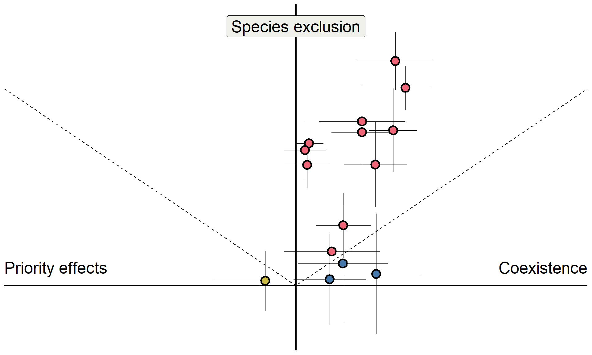
Detailed in Kandlikar et al. (2021)
Do microbes generate fitness differences in nature?
In California grasslands, microbes tend to drive stronger fitness differences than stabilization.
Can we answer this question more generally?


Results in Yan, Levine, and Kandlikar (2022); Analyses available on Zenodo

Microbially-mediated intransitivity in pine-oak forests in Spain, Pajares-Murgó et al. (2024)
Gradients in soil moisture from forest edge to interior

Gradients in soil moisture from forest edge to interior

Gradients in soil moisture from forest edge to interior

Detailed in Krishnadas et al. (2018)
Can variable plant–soil feedback explain this result?

Quantify pairwise plant–soil feedback under high and low water conditions in a shadehouse

Exaggerated microbially mediated fitness differences in dry soils could contribute to erosion of diversity at fragment edges.
Analyses ongoing
Applications of basic ecology to habitat management

PhD student
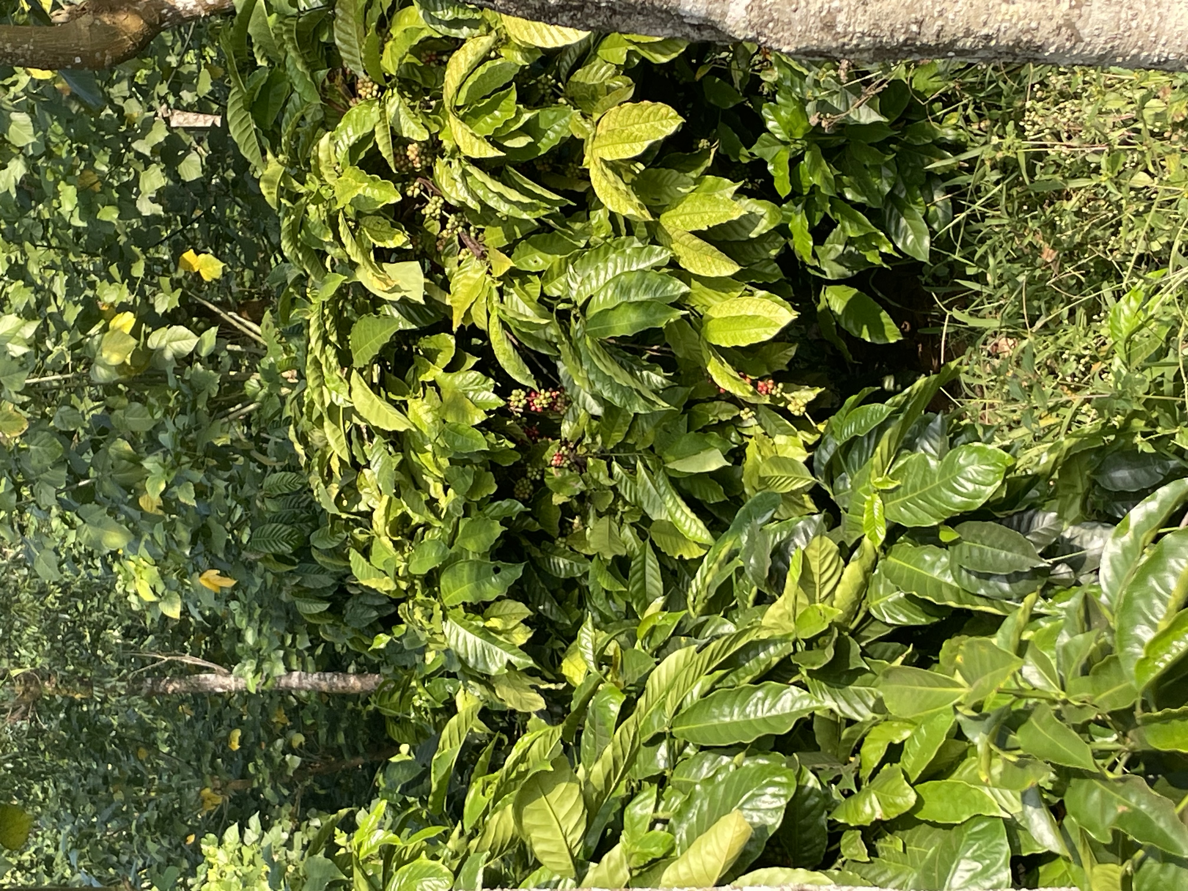
Do soil microbes contribute to invasion of coffee into forest edges?
Do soil microbes in abandoned coffee orchards affect restoration?
Applications of basic ecology to habitat management
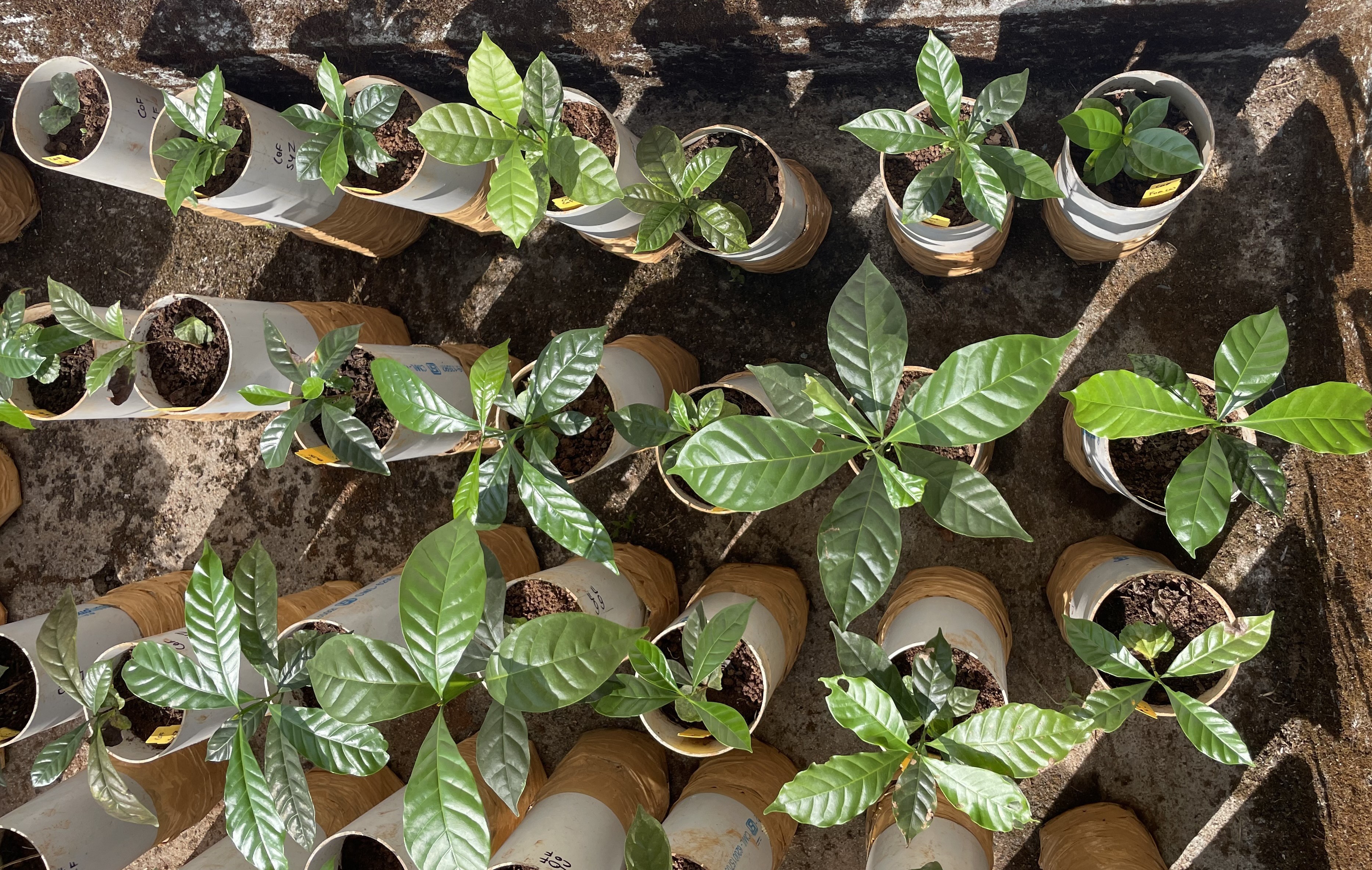
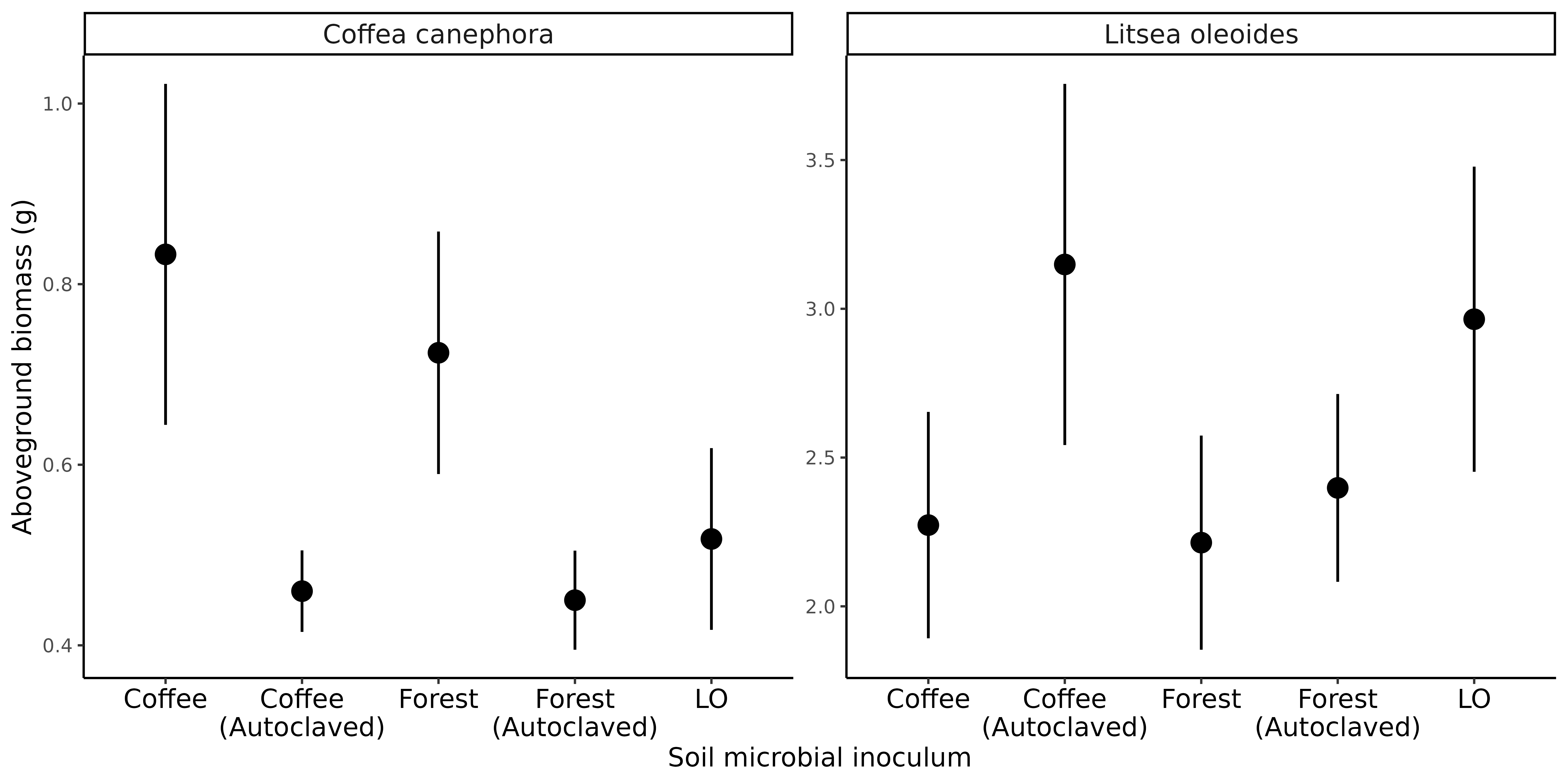
Extremely preliminary analyses!
Coffee growth enhanced by forest soil microbes
Microbes in coffee soil suppress growth of native seedlings
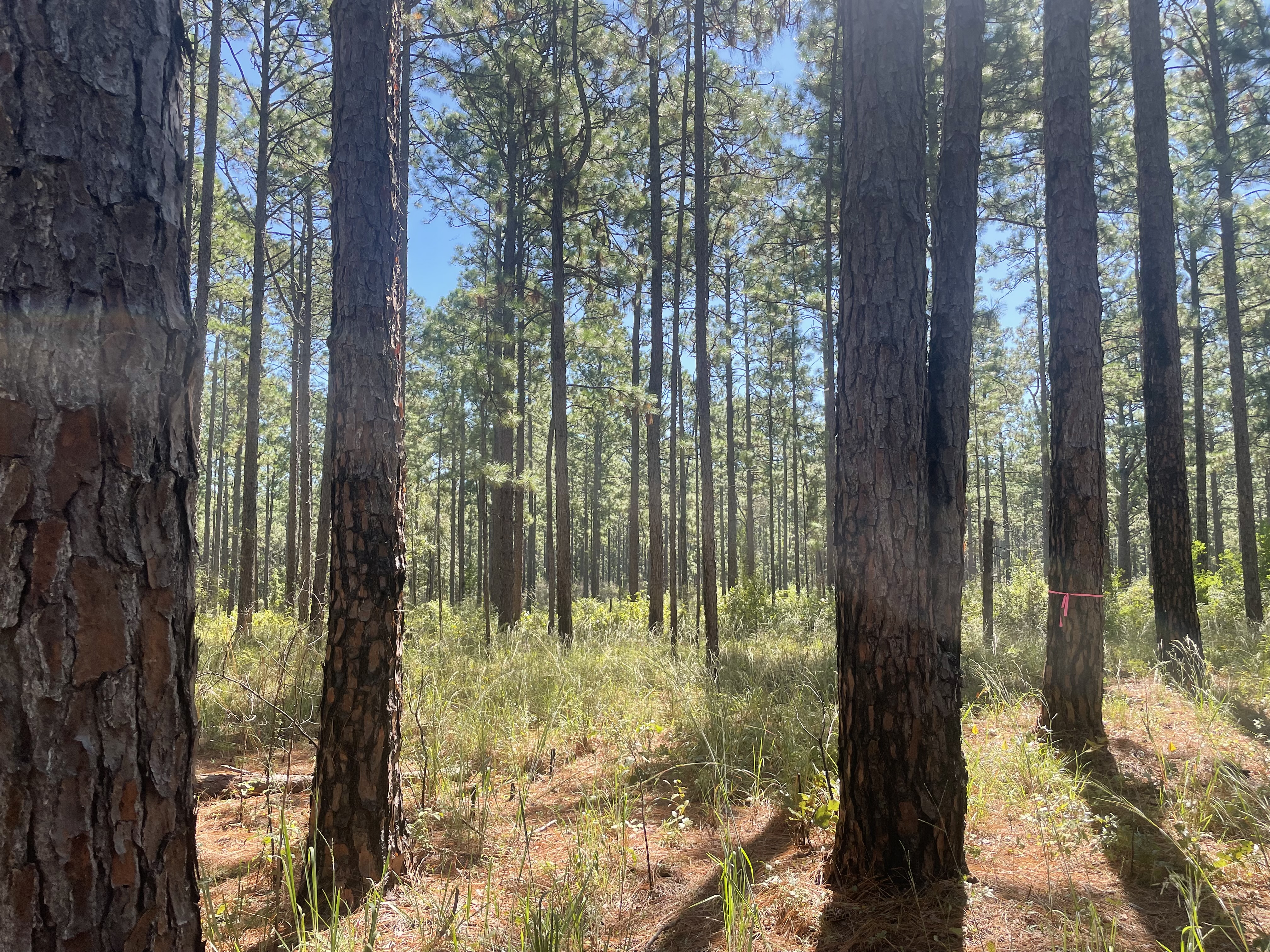
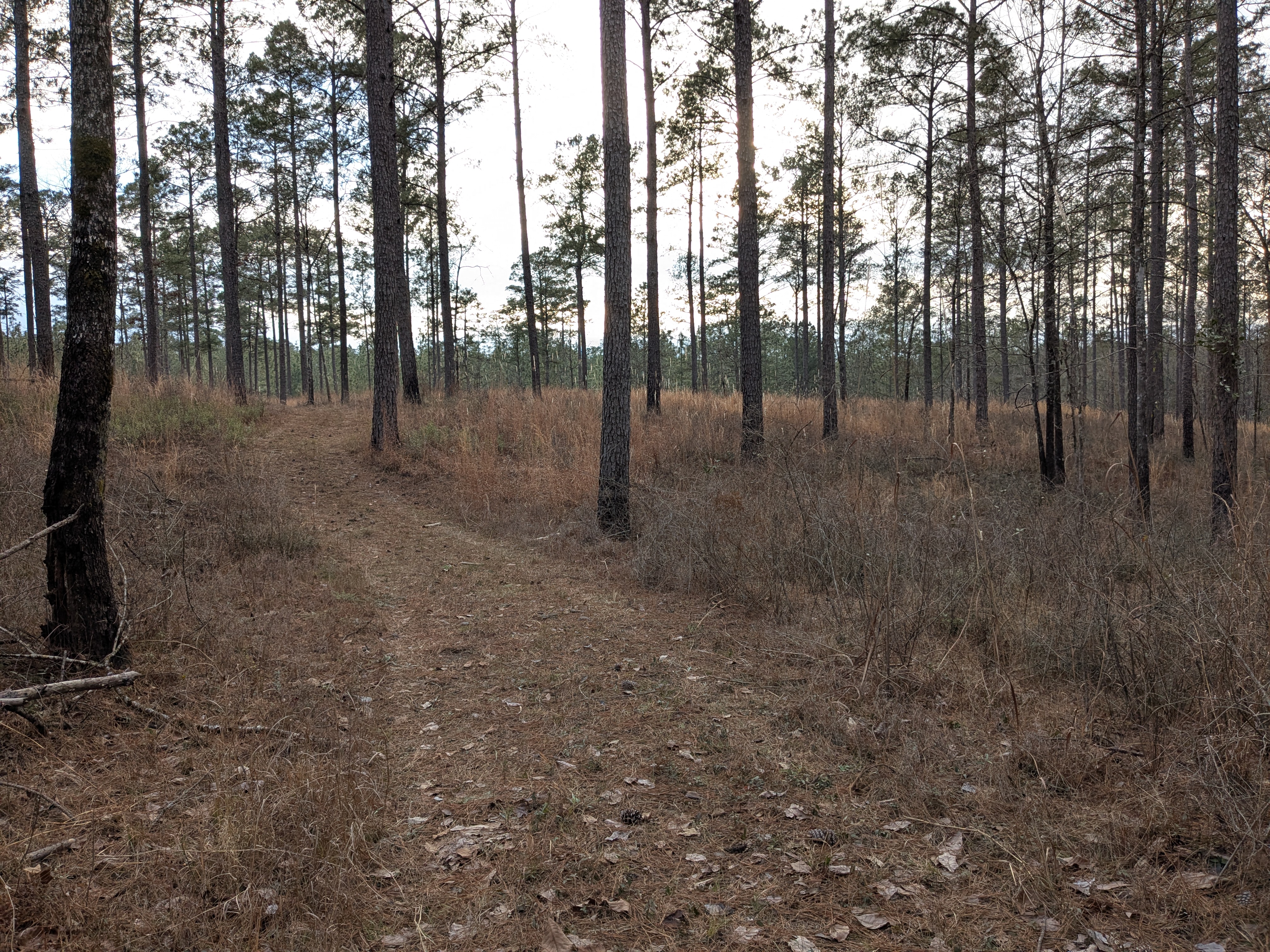
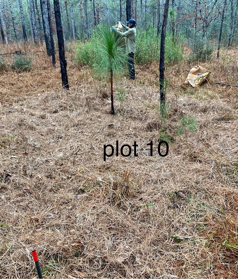
Longleaf pine savanna understory at Palustris Experimental Forest
Across ecosystems, grasses tend to experience negative feedback
Code
# curl::curl_download("https://datadryad.org/downloads/file_stream/2789266", destfile = "../data/jiang2024-dataset.csv")

jiang_dat <- read_csv("../data/jiang2024-dataset.csv")


# jiang_metamod  <- metafor::rma.mv(rr, var, data = jiang_dat,   mods = ~ Life.form-1)
# saveRDS(jiang_metamod, "../data/jiang-metamod.rds")

metamod <- readRDS("../data/jiang-metamod.rds")

metamod_s <- broom::tidy(metamod)

jiang_dat |>
  ggplot(aes(x = rr, y = Life.form, color = Life.form)) +
  ggbeeswarm::geom_quasirandom(shape = 21) +
  scale_color_manual(values = c("#ccbb44","#228833")) +
  annotate("point",
           x = metamod_s$estimate[1], y = 1, size = 3, shape = 21, stroke = 1.5) +
  annotate("point",
           x = metamod_s$estimate[2], y = 2, size = 3, shape = 21, stroke = 1.5) +
  ylab("") +
  xlab("Growth in self vs. growth in non-self") +
    xlim(-2.5,2.5)+
  geom_vline(xintercept = 0, linetype = 'dashed') +
  theme(legend.position = "none",
        axis.text.y = element_text(size = 12, color = 'black'))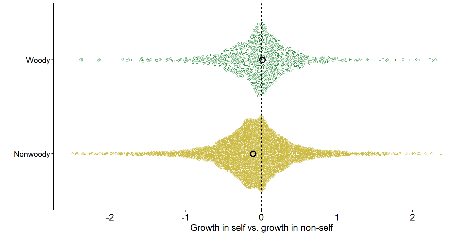
Data from Jiang et al. (2024)
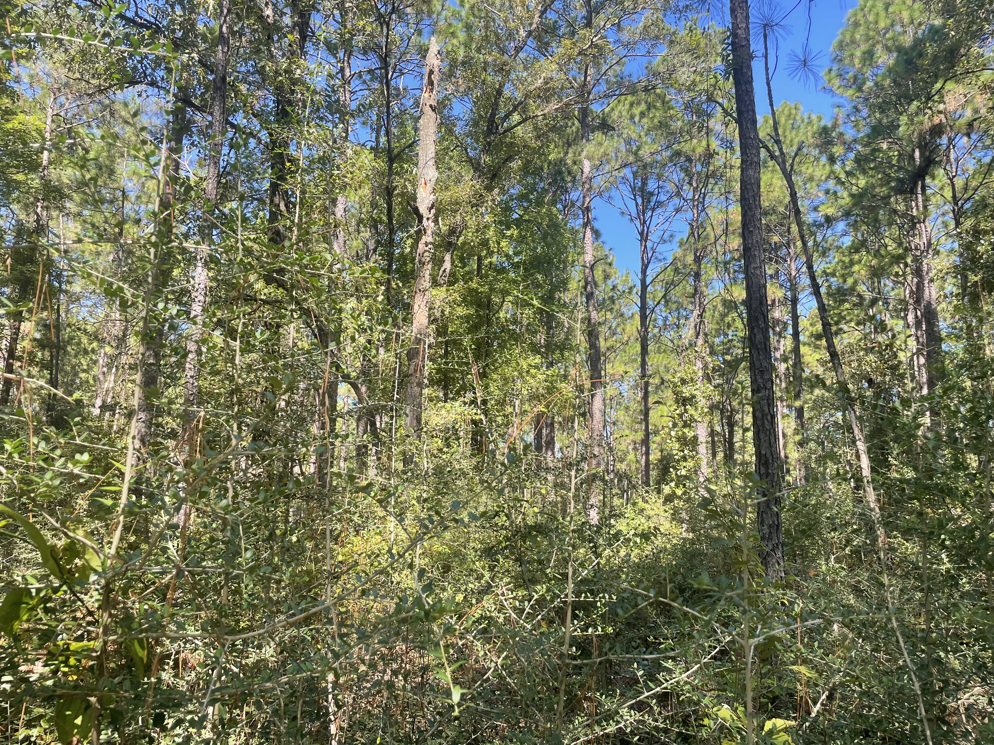
Do soil microbes play a role in driving shrubification under fire suppression?
What are the direct impacts of fire on soil microbial dynamics?
Does the history and severity of fire mediate the impact of soil microbes on plant performance and coexistence?

Postdoc
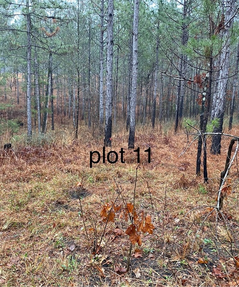
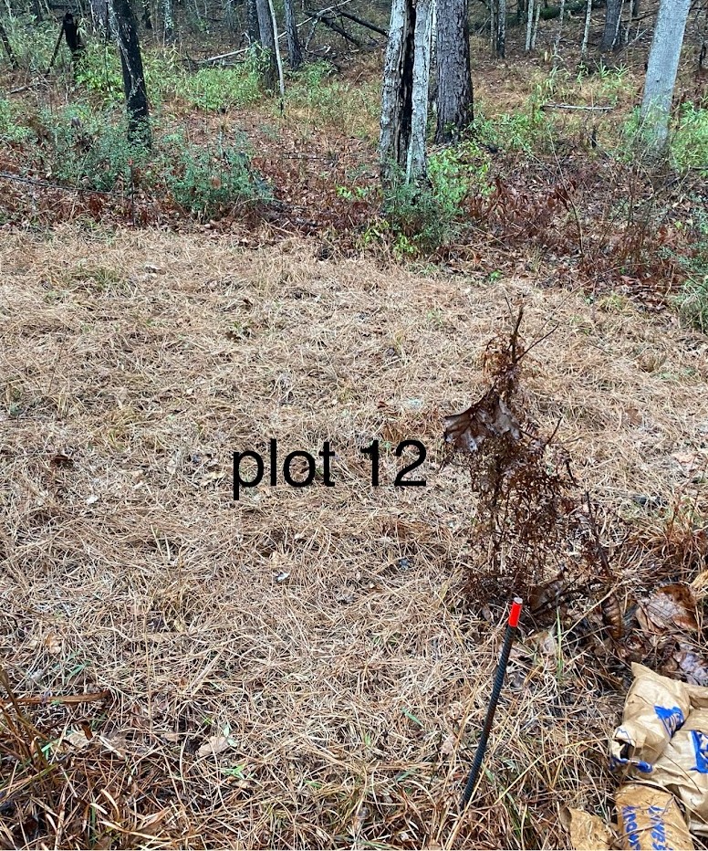
Plot set to burn next week
How does burn severity affect biotic and abiotic soil properties?
What are the dynamics of recovery?
Mathematical modeling of plant dynamics

- Goal: translate results from short-term experiments into long-term projections of community dynamics
Past work: Soil microbial legacies mediate plant response to drought across generations
Code
# curl::curl_download("https://datadryad.org/downloads/file_stream/50543", destfile = "../data/lau2012-dataset.csv")

lau_dat <- read_csv("../data/lau2012-dataset.csv")
lau_dat |>
  group_by(Contemp_Water, Plant_History, Microbe_History) |>
  filter(!is.na(Fruit_number)) |>
  summarize(mean_fruit = mean(Fruit_number),
            sd_fruit = sd(Fruit_number),
            nreps = n(),
            sem = sqrt(sd_fruit/(nreps-1))) |>
  mutate(Microbe_History =
           ifelse(Microbe_History == "Dry microbes", "Dry-adapted\nmicrobes", "Wet-adapted\nmicrobes")) |>
  filter(Plant_History == "Wet") |> # Only show wet history plants for simplicity
  ggplot(aes(x = Contemp_Water, y = mean_fruit,
             ymin = mean_fruit-sem,
             ymax = mean_fruit+sem,
             fill = Microbe_History)) +
  geom_pointrange(shape = 21,
                  size = 1.25,
                  linewidth = 1,
                  position = position_dodge(width = 0.25)) +
  scale_fill_manual(name = "",
                      values = c("#cfe2f3ff", "#0b5394ff")) +
  scale_y_continuous(#limits = c(0,6),
                     name = "Fruit number") +
  xlab("Contemporary watering") +
  # facet_wrap(.~Plant_History, scales = "free") +f
  theme(axis.text = element_text(size = 12, color = "black"),
        legend.text = element_text(size = 12),
        legend.position = "inside",
        legend.position.inside = c(0.8,0.2),
        legend.background = element_rect(color = "black"))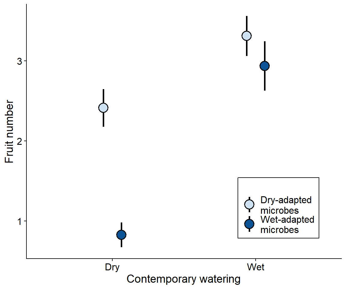
Brassica rapa’s tolerance of dought is enhanced by growing with a drought-adapted soil microbiome Data from Lau and Lennon (2012)
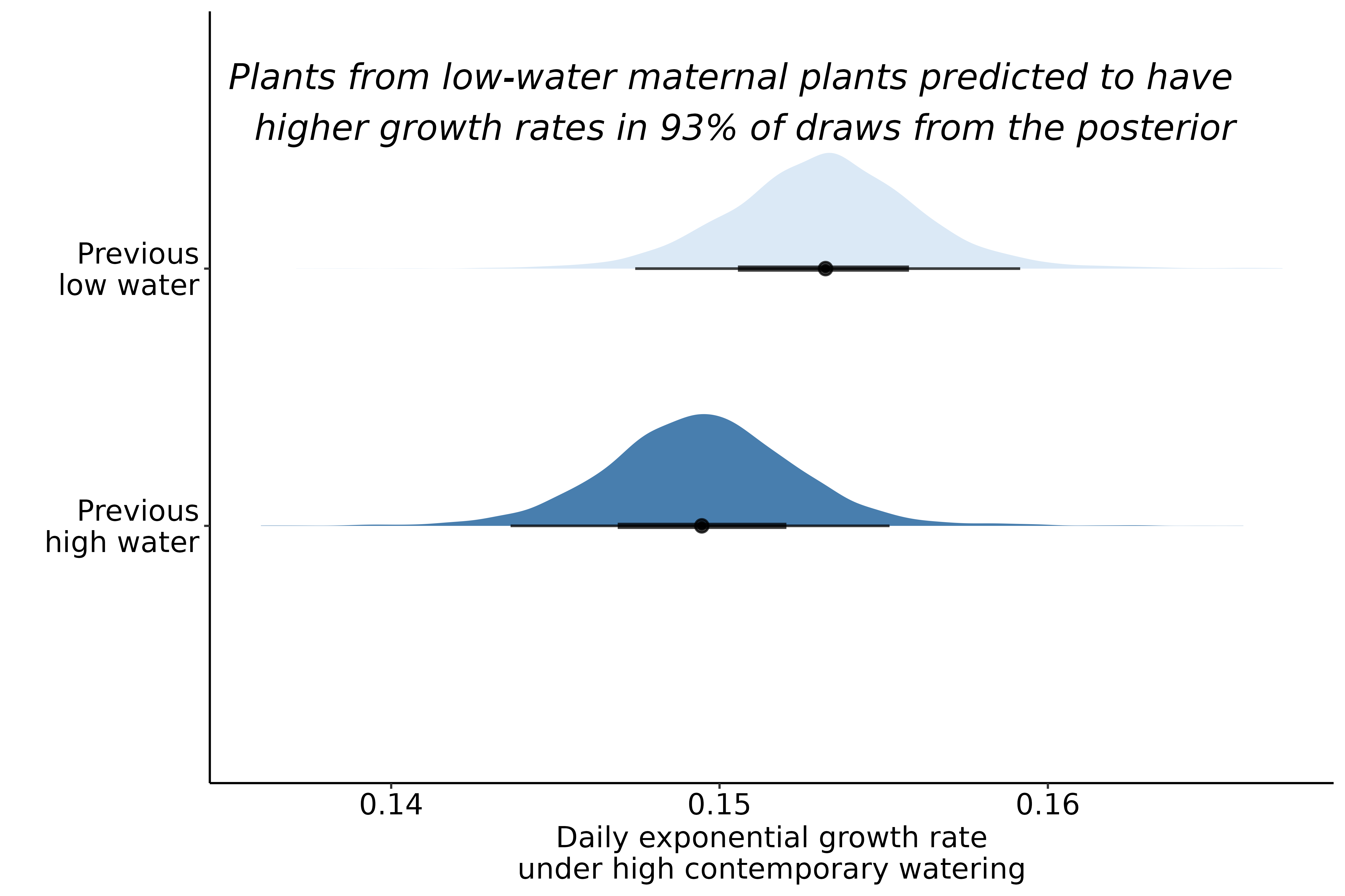
Ongoing/future work: What is the mechanistic basis, and how commonly do microbes shape transgenerational plant dynamics under abiotic stress?
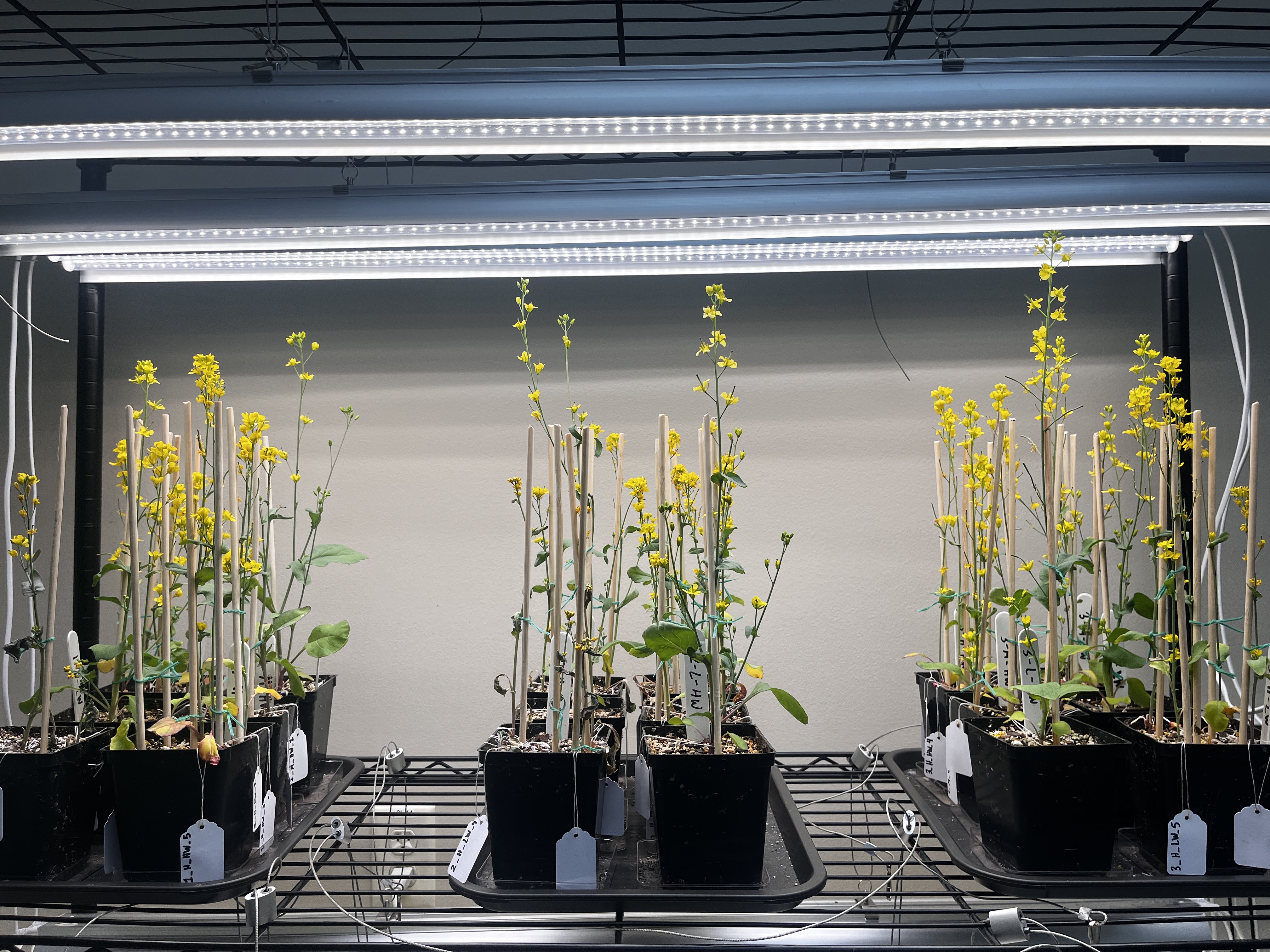

Postbac Scholar


Currently in the second generation of experimental drought, with additional plants grown to evaluate immediate maternal effects on plant functional traits
Drought imposes a fitness cost to B. rapa

Extremely preliminary analyses!
Drought imposes a fitness cost to B. rapa
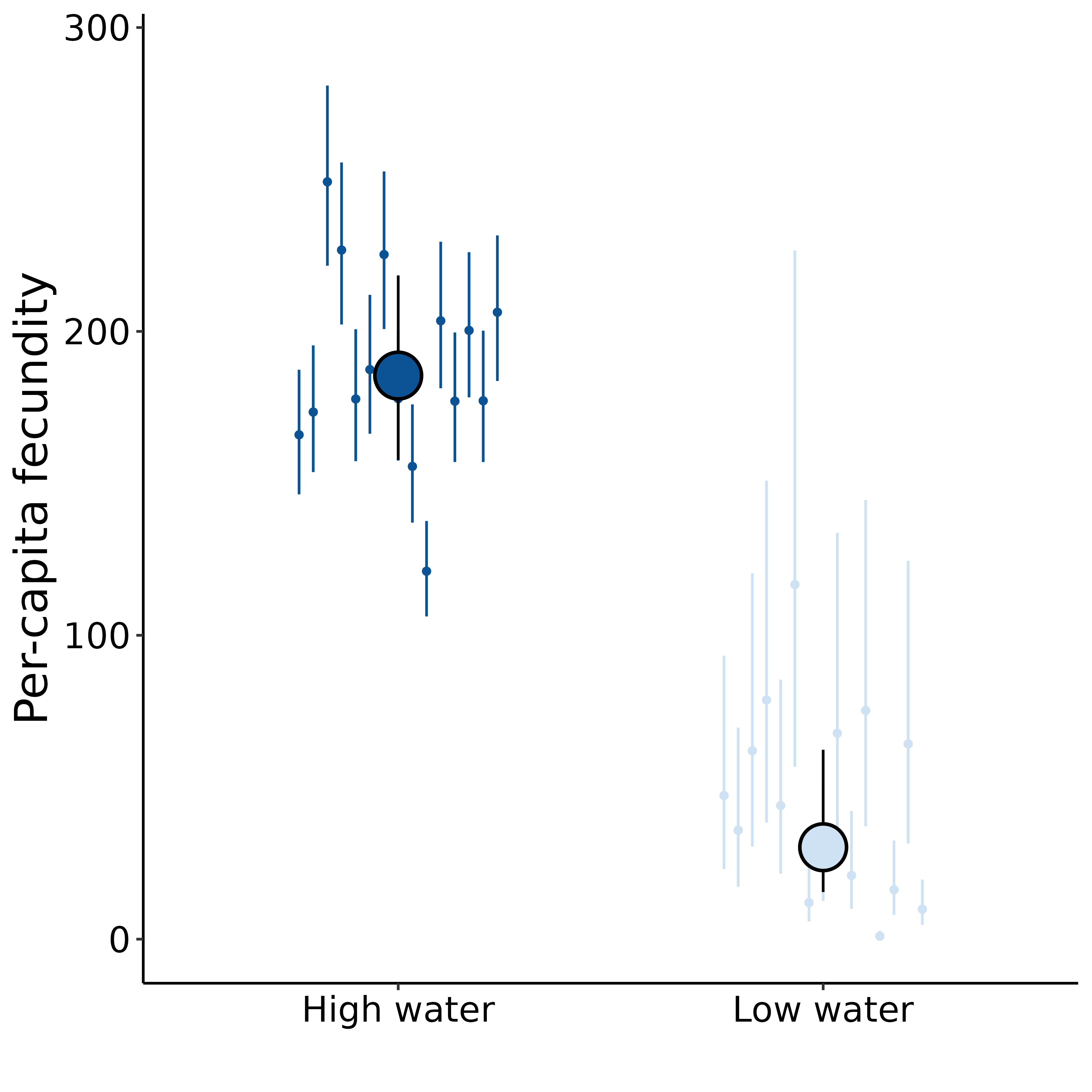
Extremely preliminary analyses!
Drought imposes a fitness cost to B. rapa
Evidence of genetic variation in drought tolerance
Extremely preliminary analyses!
Currently in the second generation of experimental drought, with additional plants grown to evaluate immediate maternal effects on plant functional traits
Early indication of maternal effects
Extremely preliminary analyses!
Other projects in the lab

PhD student
How does nutrient enrichment structure plant–mycorrhizal symbiosis?

PhD student
Citizen science for invasion ecology